Advanced Macroeconomics III (Galí)

Preface by Lorenzo Bianchi Chignoli

These lecture notes were originally prepared for the Advanced Macroeconomics III course offered by Jordi Galí in the PhD in Economics program at Universitat Pompeu Fabra during the Spring 2025 term. The content is primarily derived from my personal notes from Jordi Galí’s lectures, complemented by key excerpts from his textbook Monetary Policy, Inflation, and the Business Cycle (Galí, 2015, 2nd ed.). Many of the mathematical derivations were worked out as exercises and, therefore, may contain inaccuracies. I would like to extend my special thanks to Vincent D’Anzi and Lorenzo Marzano for their feedback and for identifying several typos. Responsibility for all remaining errors is entirely my own.

Classical Monetary Model

This section introduces a model of money in the classical economy. Most of the attending results are dramatically at odds with empirical evidence. However, this model serves as a smooth introduction to monetary economics, and to some of the notation that will be carried over hereafter. Some of the assumptions of the classical model are, indeed, quite heroic. The main assumptions are mentioned below:

• Perfect competition. To begin with, perfect competition is assumed both in the final good(s) and labor markets. Perfect competition implies that all agents are price takers in all markets, and (rightfully) believe they can sell as many goods as they are demanded at the given wage or price.
• Market clearing. Prices and wages adjust continuously to allow for market clearing (although the mechanism for such adjustment, remains, as usual, entirely unexplained).
• Homogeneous representative agent. Heterogeneity is ignored and a representative household is considered for simplicity.
• Money in the utility function. In this model, money enters the utility function directly. There are several ways to model money demand. In the baseline model, the convenient approach is simply to assume that money holdings provide some services, reflected in the utility function: money figures in the utility function directly, as a transactions facilitator. This means that no utility is derived from “being rich”, although some recent expansions of the model have included such specifications (the so called “rough utility function”). Put simply, its role may be justified theoretically as a sort of “lubricant” for transactions. However, in the continuation of the chapter, some alternative approaches to include money in the household problem will be explored.
• Labor economy. For simplicity, the entire course assumes no capital accumulation and no investment (labor is the only input).
• Closed economy.

Optimality

This section considers a representative household with a general (neoclassical) utility function and derives the optimality conditions in the most generic case. Later on, a specific form for this functions will be introduced — namely, the CRRA utility function. As for money demand,

Consider the utility objective function ${\mathbb{E}}_0{\sum }_{t=0}^{\infty }{\beta }^{t}U(C_t,N_t,L_t;Z_t)$, where $N_t$ indicates hours of work (or number of workers per household). $L_t$ denote the real balances, that is to say the real value of moneyholdings: $L_t\equiv \frac{M_t}{P_t}$. As usual, $\beta =e^{-\rho }$, and $Z_t$ is a preference shock. Utility is neoclassical, and the budget constraint is:

$$P_t{C}_t+Q_t{B}_t+M_t\le B_{t-1}+M_{t-1}+W_t{N}_t+P_t{D}_t-P_t{T}_t$$

where $Q_t$ is the return of a one-period riskless bond $B_t$ with yield defined as $Q_t\equiv e^{-i_t}$ for some nominal interest rate $i_t$. In this economy, households own equity of the firms, and dividends $D_t$ denote real dividends (whenever a quantity is premultiplied by prices, is to obtain nominal balance). Note that households are homogeneous, and therefore shares owned per household can be ignored. To prevent households to borrow indefinitely, that is issuing infinite ${\lim }_{T\to \infty }{Q}_T=-\infty$ instead of buying bonds and repaying the debt with new issuance (Ponzi scheme), impose the solvency constraint:

$$\underset{T\to \infty }{\lim }{\mathbb{E}}_t\{{\Lambda }_{t,t+T},{\mathcal{A}}_{t+T}\}\ge 0$$

where ${\mathcal{A}}_t\equiv \frac{B_{t-1}+M_{t-1}}{P_t}$ is total financial wealth, while ${\Lambda }_{t,t+T}\equiv {\beta }^T\frac{U_{c,t+T}}{U_{c,t}}$ is the stochastic discount factor. This is the minimal assumption to prevent Ponzi schemes. Since ${\Lambda }_{t,t+T}$ will be decreasing as $T$ increases, it implies that household debt cannot increase at a higher rate than the interest rate. Trade in equity could be theoretically included, but households are homogeneous and therefore no trade occurs in equilibrium.

No-Ponzi condition

In this focus, we’ll try to understand why the no-Ponzi condition takes that specific form. The derivation is a (significantly) simplified version of Woodford (2003, pp. 64-72).

The flow budget constraint above relies on the assumption of complete financial markets, i.e. markets that are completely spanning individual households’ uncertainty about future shocks. This assumption is crucial as it guarantees the existence of a unique stochastic discount factor that can be used to price any stream of future payoffs, simplifying the household’s problem significantly. While this course involves a production economy, let us adopt a more general notation also applicable to endowment economies. The flow budget constraint can be rewritten as $P_t{C}_t+Q_t{B}_t\le B_{t-1}+Y_t$ (money is absent, as if we’re in the cashless limit of a monetary economy). Assume a natural borrowing limit. A household is solvent if its financial assets $B_t$ are sufficient to cover all its net liabilities: It cannot borrow more than the present value of its entire future stream of non-financial income. Then:

$$B_t\ge -\sum _{T=t+1}^{\infty }{\mathbb{E}}_{t+1}[Q_{t+1,T}{Y}_T]$$

Note that the notation $Q_{t+1,T}$ is not casual: this denotes the nominal stochastic discount factor, which is exactly the random variable used to price at time $t+1$ any asset with return equal to 1 at $T$ (in the case of bonds, $Q_t={\mathbb{E}}_t[Q_{t,t+1}]$). To continue, iterate the standard flow budget constraint from period $t$ to some future period $T$, obtaining the finite-horizon budget constraint:

$$\sum _{s=t}^T{\mathbb{E}}_t[Q_{t,s}{P}_s{C}_s]+{\mathbb{E}}_t[Q_{t-T}{B}_T]=B_{t-1}+\sum _{s=t}^T{\mathbb{E}}_t[Q_{t,s}{Y}_s]$$

Continue by taking the infinite-horizon limit:

$$\underset{T\to \infty }{\lim }{\mathbb{E}}_t[Q_{t,T}{B}_T]\ge 0$$

that is, the expected present value of the household’s financial assets in the infinitely distant future cannot be negative. Define the real stochastic discount factors as the nominal stochastic discount factor adjusted for prices, ${\Lambda }_{t,T}=Q_{t,T}\frac{P_T}{P_t}$. Thus:

$$\begin{array}{rl}\underset{T\to \infty }{\lim }{\mathbb{E}}_t\left[\left({\Lambda }_{t,T}\frac{P_t}{P_T}\right)B_T\right]& \ge 0\\ P_t\underset{T\to \infty }{\lim }{\mathbb{E}}_t\left[{\Lambda }_{t,T}\frac{B_T}{P_T}\right]& \ge 0\\ \underset{T\to \infty }{\lim }{\mathbb{E}}_t\left[{\Lambda }_{t,T}\frac{B_T}{P_T}\right]& \ge 0\end{array}$$

which is equivalent to the original equation (after the addition of cash).

There are three optimality conditions, which will be derived below:

$$\{\begin{array}{l}-\frac{U_{n,t}}{U_{c,t}}=\frac{W_t}{P_t}\\ Q_t=\beta {\mathbb{E}}_t\left\{\frac{U_{c,t+1}}{U_{c,t}}\frac{P_t}{P_{t+1}}\right\}\\ \frac{U_{m,t}}{U_{c,t}}=1-Q_t=1-e^{-i_t}\end{array}$$

Government Budget Constraint

Note that, if a public sector were to be introduced, this model should also satisfy the government budget constraint:

$$P_t{G}_t+B_{t-1}^G=P_t{T}_t+Q_t{B}_t^G+\Delta M_t$$

which implies a fiscal policy rule determining $\{G_t,B_t^G,T_t\}$ and a monetary policy rule determining $\{M_t,i_t\}$. The implicit assumption throughout this section is that $G_t=0$.

For the derivation, assume the household follows an optimal plan and consider deviations for such plan. Provided that the plan was optimal in the first place, deviations must necessarily decrease utility. This method is usually referred to as the variational approach and can be very handy in solving optimality conditions along multiple variables. First, consider deviations in consumption and labor, that is satisfying the relationship $P_{t}d{C}_t=W_{t}d{N}_t$:

$$\begin{array}{rl}{U}_{c,t}d{C}_t+U_{n,t}d{N}_t& =0\\ \left[U_{c,t}\frac{W_t}{P_t}+U_{n,t}\right]d{N}_t& =0\\ U_{c,t}\frac{W_t}{P_t}+U_{n,t}& =0\end{array}$$

The second equality follows from the fact that $P_{t}d{C}_t=W_{t}d{N}_t$: since no changes occur in the equity market, all additional income has to be spent in consumption. Moreover, perfect competition in the labor market implies that the household believes to possibly supply as much labor as they like. Thus, the terms in brackets must be 0: for negative or positive values some improvement would be possible by changing labor or consumption, violating the assumption that the household is on the optimal path — a contradiction. As a consequence, the marginal rate of substitution between consumption an labor must be equal to the wage to price ratio.

Now consider diverting consumption today with consumption tomorrow. Consider both the cases where household employs money and bonds to increase their consumption. If such deviations are performed using bonds, then it must be that $\underset{d{B}_t}{\underbrace{P_{t+1}d{C}_{t+1}}}=-\frac{P_t}{Q_t}d{C}_t$. Rearranging, this is the same as $d{C}_t=-\frac{P_{t+1}}{P_t}{Q}_{t}d{C}_{t+1}$. Therefore, factorizing $d{C}_t$:

$$\begin{array}{rl}{U}_{c,t}d{C}_t+\beta {\mathbb{E}}_t[U_{c,t+1}d{C}_{t+1}]& =0\\ \left[U_{c,t}-\frac{1}{Q_t}\beta \mathbb{E}{U}_{c,t+1}\frac{P_t}{P_{t+1}}\right]d{C}_t& =0\\ U_{c,t}-\frac{1}{Q_t}\beta \mathbb{E}{U}_{c,t+1}\frac{P_t}{P_{t+1}}& =0\end{array}$$

Finally, consider such deviations using money, that is satisfying $\underset{d{M}_t}{\underbrace{P_{t+1}d{C}_{t+1}}}=-P_{t}d{C}_t$. Rearranging, this is the same as $d{C}_t=-\frac{P_{t+1}}{P_t}d{C}_{t+1}$. Also recall that, by definition, $L_t=\frac{M_t}{P_t}$, and thus it must be that $d{L}_t=\frac{d{M}_t}{P_t}$. Plugging in these two results, note that:

$$\begin{array}{rl}{U}_{c,t}d{C}_t+U_{l,t}dLt+\beta \mathbb{E}[U_{c,t+1}d{C}_{t+1}]& =0\\ U_{c,t}d{C}_t+U_{l,t}\frac{d{M}_t}{P_t}-\beta \mathbb{E}\left[U_{c,t+1}\frac{P_t}{P_{t+1}}d{C}_t\right]& =0\\ U_{c,t}d{C}_t-U_{l,t}d{C}_t-\beta \mathbb{E}\left[U_{c,t+1}\frac{P_t}{P_{t+1}}d{C}_t\right]& =0\\ \left(U_{c,t}-U_{l,t}-\beta \mathbb{E}\left[U_{c,t+1}\frac{P_t}{P_{t+1}}\right]\right)d{C}_t& =0\\ U_{c,t}-U_{l,t}-\beta \mathbb{E}\left[U_{c,t+1}\frac{P_t}{P_{t+1}}\right]& =0\\ U_{c,t}(1-Q_t)-U_{l,t}& =0\end{array}$$

where the last equality is obtained by exploiting the previous optimality condition: in fact, $\beta \mathbb{E}\left[U_{c,t+1}\frac{P_t}{P_{t+1}}\right]=-Q_t{U}_{c,t}$. This condition indicates the marginal utility of real balances must be equal to, approximately, $i_t$ (can be easily seen by doing a first-order Taylor expansion around 0). The interest rate can be interpreted as the “cost” of holding real balances, namely the opportunity cost of holding real balances in opposed to holding wealth in the form of bonds. Note that his equation only appears in models with money into the utility function.

Let us continue by specifying a structural form for households’ utility. Assume that utility has a CRRA shape (note that, for the sake of simplicity, $C$ and $L$ have the same $\sigma$ parameter), and a constant Frisch elasticity of labor $\varphi$.

$$U(C_t,N_t)=\{\begin{array}{ll}\left(\frac{C_t^{1-\sigma }-1}{1-\sigma }-\frac{N_t^{1+\varphi }}{1+\varphi }+{\Xi }_t^{\sigma }\frac{L_t^{1-\sigma }-1}{1-\sigma }\right)Z_t& \sigma \ne 1\\ \left(\log (C_t)-\frac{N_t^{1+\varphi }}{1+\varphi }+{\Xi }_t^{\sigma }\log (L_t)\right)Z_t& \sigma =1\end{array}$$

The preference shock multiplies the entire function: in this formulation, we can interpret such shock as a pure demand shock. In some sense, it can be interpreted as equivalent to a shock to $\beta$. Other sources of shock can affect labor supply specifically (see $\Phi$ in the slides) or the money demand shock (in the slides, $\Xi$). Another important assumption is that the impact of real balances is separable. This not innocuous assumption means that the marginal utility of consumption and the marginal disutility of labor do not depend on real balances: $L_t\perp \frac{U_{n,t}}{U_{c,t}}$. By plugging in the specific derivatives of the functional form is the utility function leads to the implied optimality conditions:

$$\{\begin{array}{ll}\frac{W_t}{P_t}& =C_t^{\sigma }{N}_t^{\varphi }\\ Q_t& =\beta {\mathbb{E}}_t\left\{{\left(\frac{C_{t+1}}{C_t}\right)}^{-\sigma }\left(\frac{Z_{t+1}}{Z_t}\frac{P_t}{P_{t+1}}\right)\right\}\\ L_t& =C_t(1-e^{-i_t}{)}^{-\frac{1}{\sigma }}\end{array}$$

Assume a steady state with constant inflation and no trend growth such as $Q\Pi =\beta$ which implies $i=\rho +\pi$. The corresponding log-linearized optimality conditions are:

$$\{\begin{array}{ll}{w}_t-p_t& =\sigma c_t+\varphi n_t\\ c_t& ={\mathbb{E}}_t[c_{t+1}]-\frac{1}{\sigma }(i_t-{\mathbb{E}}_t[{\pi }_{t+1}]-\rho )+\frac{1}{\sigma }(1-{\rho }_z)z_t\\ l_t& =c_t-\frac{1}{\sigma }\log (1-e^{-i_t})\\ & \approx c_t-\eta i_t+\zeta \end{array}$$

where denotes the semielasticity of money demand. In the most general form, the money demand function is postulated as equal to $m_t-p_t=c_t-\eta i_t$, where $\eta \equiv \frac{\partial (m_t-p_t)}{\partial i_t}$ is the semi-elasticity of money demand. This form is also derived in the following exercise, as the optimality condition for a utility function with direct utility from real balances. Details on the derivation of the Euler equation as a first-order approximation are outlined after the following exercise.

Household Optimality through the Lagrangian

Set up the intertemporal household maximization problem supposing CRRA utility with preferenze shocks $Z$, where $\log (Z_t)\equiv z_t=(1-{\rho }_z)z_{t-1}+{ϵ}_t$:

$$\underset{c,N}{\max }\left(\frac{C^{1-\sigma }}{1-\sigma }-\frac{N^{1+\varphi }}{1+\varphi }\right)Z+\beta \left(\frac{(C^{\prime }{)}^{1-\sigma }}{1-\sigma }-\frac{(N^{\prime }{)}^{1+\varphi }}{1+\varphi }\right)\mathbb{E}[Z^{\prime }]$$

subject to

$$\{\begin{array}{l}{P}_t{C}_t+Q_t{B}_t+M_t\le B_{t-1}+M_{t-1}+W_t{N}_t+P_t{D}_t-P_t{T}_t\\ {\lim }_{T\to \infty }\mathbb{E}\left\{{\Lambda }_{t,T}\frac{B_T}{P_T}\right\}\end{array}$$

This can be conveniently solved through a Lagrangian:

$$\begin{array}{rl}\mathcal{L}& \equiv \left(\frac{C^{1-\sigma }}{1-\sigma }-\frac{N^{1+\varphi }}{1+\varphi }\right)Z-\frac{\lambda }{P}(PC+QB+M-B_{-}-M_{-}-WN-PD+PT)\\ & +\beta \left[\left(\frac{(C^{\prime }{)}^{1-\sigma }}{1-\sigma }-\frac{(N^{\prime }{)}^{1+\varphi }}{1+\varphi }\right)Z^{\prime }-\frac{{\lambda }^{\prime }}{P^{\prime }}(P^{\prime }{C}^{\prime }+Q^{\prime }{B}^{\prime }+M^{\prime }-B-M-W^{\prime }{N}^{\prime }-P^{\prime }{D}^{\prime }+P^{\prime }{T}^{\prime })\right]\end{array}$$

where the expectation term was omitted for readibility. Note that the multipliers must be normalized by the price level. The FOCs are as follows:

$$\begin{array}{rlrl}[C]& :& Z{C}^{-\sigma }-\lambda & =0\\ [C^{\prime }]& :& Z^{\prime }(C^{\prime }{)}^{-\sigma }-{\lambda }^{\prime }& =0\\ [N]& :& -Z{N}^{\varphi }+\lambda \frac{W}{P}& =0\\ [B]& :& \frac{\lambda Q}{P}& =\beta \frac{{\lambda }^{\prime }}{P^{\prime }}\\ [M]& :& \frac{\lambda }{P}& =\frac{\beta {\lambda }^{\prime }}{P^{\prime }}\end{array}$$

Plugging $[C]$ into $[N]$ leads to the first optimality condition:

$$\frac{N^{\varphi }}{C^{-\sigma }}=\frac{W}{P}$$

while the second optimality condition follows pluggin $[C]$ and $[C^{\prime }]$ into $[B]$:

$$\begin{array}{rl}Q& =\beta \frac{{\lambda }^{\prime }}{\lambda }\frac{P}{P^{\prime }}\\ & =\beta \frac{Z^{\prime }}{Z}{\left(\frac{C}{C^{\prime }}\right)}^{\sigma }\frac{P}{P^{\prime }}\end{array}$$

Finally, we conclude the exercise by considering a generalization with (separable) money demand in the utility function.

$$\begin{array}{rl}\mathcal{L}& \equiv \left(\frac{C^{1-\sigma }}{1-\sigma }-\frac{N^{1+\varphi }}{1+\varphi }+\frac{L^{1-\nu }}{1-\nu }\right)Z-\frac{\lambda }{P}(PC+QB+M-B_{-}-M_{-}-WN-PD+PT)+\\ & +\beta \left[\left(\frac{(C^{\prime }{)}^{1-\sigma }}{1-\sigma }-\frac{(N^{\prime }{)}^{1+\varphi }}{1+\varphi }+\frac{(L^{\prime }{)}^{1-\nu }}{1-\nu }\right)Z^{\prime }-\frac{{\lambda }^{\prime }}{P^{\prime }}(P^{\prime }{C}^{\prime }+Q^{\prime }{B}^{\prime }+M^{\prime }-B-M-W^{\prime }{N}^{\prime }-P^{\prime }{D}^{\prime }+P^{\prime }{T}^{\prime })\right]\\ [M]& :{\left(\frac{M}{P}\right)}^{-\nu }-\frac{\lambda }{P}+\frac{\beta {\lambda }^{\prime }}{P^{\prime }}=0\end{array}$$

The money demand optimality condition is obtained plugging in $[C]$ and $[C^{\prime }]$ for the multipliers:

$$\begin{array}{rl}{L}^{-\nu }& =C^{-\sigma }Z-\beta \frac{(C^{\prime }{)}^{-\sigma }{Z}^{\prime }}{P^{\prime }}\\ \frac{L^{-\nu }}{C^{-\sigma }Z}& =1-\beta {\left(\frac{C^{\prime }}{C}\right)}^{-\sigma }\frac{Z}{Z^{\prime }}\frac{P}{P^{\prime }}\\ \frac{L^{-\nu }}{C^{-\sigma }Z}& =1-Q\\ & =1-e^{-i_t}\end{array}$$

which corresponds to the formula present in the textbook, namely $U_{l,t}=U_{c,t}(1-e^{-i_t})$.

As proposed thereof, the first-order Taylor expansion $\log (1-e^{-i_t})\sim \text{const.}+\frac{1}{e^{i_t}-1}{i}_t$ can be used to approximate the log-linear form (up to an uninteresting constant) as $m_t-p_t=\frac{\sigma }{\nu }{c}_t-\eta i_t$, where $\eta \equiv \frac{1}{\nu (e^{i_t}-1)}\simeq \frac{1}{\nu i_t}$ is the implied interest semielasticity of money demand. This can be noticed by expanding the last term of:

$$m_t-p_t=\frac{\sigma }{\nu }{c}_t-\frac{1}{\nu }\log (1-e^{-i_t})$$

Take a first order expansion by noting the the first derivative of $\log (1-e^{-i_t})$ is equal to $\frac{e^{-i_t}}{1-e^{-i_t}}=\frac{1}{e^{i_t}-1}$. Therefore, the first-order Taylor expansion of the loglinear equation around some $i$ yields:

$$\begin{array}{rl}\log (1-e^{-i_t})& \approx \log (1-e^{-i_t})+\frac{1}{e^{i_t}-1}(i_t-i)\\ & =\left[\underset{\text{constant}}{\underbrace{\log (1-e^{-i})+\frac{i}{e^i-1}}}\right]+\frac{i_t}{e^i-1}\end{array}$$

This can plugged into the original equation:

$$m_t-p_t\approx \frac{\sigma }{\nu }{c}_t-\left(\frac{1}{\nu (e^i-1)}\right)i_t+\text{constant}$$

which identifies $\eta \equiv \frac{1}{\nu (e^i-1)}$. Also note that, for small $i$, then $e^i-1\approx i$, so that $\eta \approx \frac{1}{\nu i}$.

To find the intertemporal Euler equation espressed in terms of the interest rate, take the optimality condition for $Q_t$ in logs:

$$\begin{array}{rl}{Q}_t& ={\mathbb{E}}_t\left[\beta \frac{Z^{\prime }}{Z}{\left(\frac{C}{C^{\prime }}\right)}^{\sigma }\frac{P}{P^{\prime }}\right]\\ 1& =\frac{{\mathbb{E}}_t\left[\beta \frac{Z^{\prime }}{Z}{\left(\frac{C}{C^{\prime }}\right)}^{\sigma }\frac{P}{P^{\prime }}\right]}{Q_t}\\ 0& =\log \left({\mathbb{E}}_t\left[\beta \frac{Z^{\prime }}{Z}{\left(\frac{C}{C^{\prime }}\right)}^{\sigma }\frac{P}{P^{\prime }}\right]\right)+i_t\\ 0& \approx i_t-\rho +{\mathbb{E}}_t[\Delta z_{t+1}]-\sigma {\mathbb{E}}_t[\Delta c_{t+1}]-{\mathbb{E}}_t[{\pi }_{t+1}]\\ \sigma {\mathbb{E}}_t[\Delta c_{t+1}]& \approx i_t-{\mathbb{E}}_t[{\pi }_{t+1}]-\rho +{\mathbb{E}}_t[\Delta z_{t+1}]\\ {\mathbb{E}}_t[\Delta c_{t+1}]& \approx \frac{1}{\sigma }(i_t-{\mathbb{E}}_t[{\pi }_{t+1}]-\rho +{\mathbb{E}}_t[\Delta z_{t+1}])\\ {\mathbb{E}}_t[c_{t+1}-c_t]& \approx \frac{1}{\sigma }(i_t-{\mathbb{E}}_t[{\pi }_{t+1}]-\rho +{\mathbb{E}}_t[z_{t+1}-z_t])\\ {\mathbb{E}}_t[c_{t+1}]-c_t& \approx \frac{1}{\sigma }(i_t-{\mathbb{E}}_t[{\pi }_{t+1}]-\rho +{\mathbb{E}}_t[z_{t+1}]-z_t)\\ c_t& \approx {\mathbb{E}}_t[c_{t+1}]-\frac{1}{\sigma }(i_t-{\mathbb{E}}_t[{\pi }_{t+1}]-\rho +{\mathbb{E}}_t[x_{t+1}]-z_t)\\ c_t& \approx {\mathbb{E}}_t[c_{t+1}]-\frac{1}{\sigma }(i_t-{\mathbb{E}}_t[{\pi }_{t+1}]-\rho -(1-{\rho }_z)z_t)\end{array}$$

where the fourth line introduces a first-order approximation (by Jensen’s inequality), as the logarithm is moved within the expectation.

Certainty-Equivalent First-Order Approximation

This Focus details why the common approximation $\mathbb{E}[f(X)]\approx f(\mathbb{E}[X])$ is a first-order Taylor approximation. We analyze the relationship by performing a Taylor expansion of the function $f(X)$ around the mean of $X$, denoted as $\mu =\mathbb{E}[X]$. The variance is ${\sigma }^2=\mathbb{E}[(X-\mu {)}^2]$. The term $f(\mathbb{E}[X])$ is exactly $f(\mu )$. The term $\mathbb{E}[f(X)]$ is analyzed by expanding $f(X)$ inside the expectation:

$$\begin{array}{rl}f(X)& \approx f(\mu )+f^{\prime }(\mu )(X-\mu )+\frac{1}{2}{f}^{\prime \prime }(\mu )(X-\mu {)}^2\\ \mathbb{E}[f(X)]& \approx \mathbb{E}\left[f(\mu )+f^{\prime }(\mu )(X-\mu )+\frac{1}{2}{f}^{\prime \prime }(\mu )(X-\mu {)}^2\right]\\ \mathbb{E}[f(X)]& \approx f(\mu )+f^{\prime }(\mu )\mathbb{E}[X-\mu ]+\frac{1}{2}{f}^{\prime \prime }(\mu )\mathbb{E}[(X-\mu {)}^2]\\ \mathbb{E}[f(X)]& \approx f(\mu )+\frac{1}{2}{f}^{\prime \prime }(\mu ){\sigma }^2\end{array}$$

A first-order (or certainty equivalent) approximation deliberately ignores all second-order and higher terms. By truncating the expansion after the first-order term, the variance term disappears:

$$\mathbb{E}[f(X)]\approx f(\mu )+f^{\prime }(\mu )\underset{=0}{\underbrace{\mathbb{E}[X-\mu ]}}=f(\mu )$$

This leads to the final result:

Certainty Equivalence First-Order Approximation

At the first order, $f(\mathbb{E}[X])$ and $\mathbb{E}[f(X)]$ are approximately equal because we intentionally ignore the term that captures the effect of variance. $f(\mathbb{E}[X])=f(\mu )\approx \mathbb{E}[f(X)]$

The ignored term, $\frac{1}{2}{f}^{\prime \prime }(\mu ){\sigma }^2$, is the “gap” explained by Jensen’s Inequality. For a concave function like $\log$, $f^{\prime \prime }(X)<0$, which explains why $\mathbb{E}[\log (X)]\le \log (\mathbb{E}[X])$. Setting this term to zero is the mathematical basis of the approximation.

The effects of the two exogenous shocks on equilibrium values are different. On the one hand, $z_t$ only affects the real interest rate $r_t$. In contrast, technology has an ambiguous effect on employment depending on $\sigma$: if it is less than 1, increasing technology increases unemployment. In fact, for larger output, a low sigma entails a small increase in consumption, which does not offset the increase in labor demanded. This can be observed by taking the log-linear optimality condition of the firm, which solves profit maximization at the given technology:

$$w_t-p_t=a_t-\alpha n_t+\log (1-\alpha )$$

(the identity of total output on the RHS and real demand on the LHS holds by market clearing). This highlights how prices depend on marginal costs: $p_t={\psi }_t\equiv w_t-[a_t-\alpha n_t+\log (1-\alpha )]$.

Real and Nominal Interest Rates

A clarification on real and nominal rates. Recall that:

• $\beta :=e^{\rho }$
• $Q_t=e^{-i_t}$ Put simply, a bond with price $Q$ which yields 1 has a return $\frac{1}{Q}$. Moreover, define:
• ${\Pi }_t:=\frac{P_{t+1}-P_t}{P_t}$ as the gross rate of inflation
• $R=\frac{1}{\beta }$ as the real neutral interest rate Since $Q$ is pinned down by $i$, the real interest rate should be equal to the returns on bonds net of inflation: $R=\frac{\frac{1}{Q}}{\Pi }$. Taking the logs, $r=-\log Q-\pi$, which is also equal to the familiar $r=i-\pi$.

As a possible interpretation of this relation, note that pure consumption smoothing can be achieved only if the real interest rate equalizes the discount rate. Deviations depend on the value of the real interest rate. How this is realized in practice is beyond the scope of this section: in the future, central banks may allow individuals to hold deposits directly through CBDC, and presumably earn interests on liquidity. A more detailed treatment of CBDC and crypto is contained in Benigno (2025).

Equilibrium

An equilibrium for the Classical model is a steady state clearing markets for goods, labor, and assets at the given technology¹:

$$\{\begin{array}{ll}{y}_t& =c_t\\ & \\ \sigma c_t+\varphi n_t& =w_t-p_t\\ & =a_t-\alpha n_t+\log (1-\alpha )\\ & \\ m_t-p_t& =l_t\\ & =c_t-\eta i_t\\ & \\ y_t& =a_t+(1-\alpha )n_t\end{array}$$

The previous conditions allow to solve endogenous variables for the exogenous variables and parameters:

$$\{\begin{array}{l}{n}_t=\frac{1-\sigma }{\sigma (1-\alpha )+\alpha +\varphi }{a}_t+\frac{\log (1-\alpha )}{\sigma (1-\alpha )+\alpha +\varphi }\equiv {\psi }_{na}{a}_t+n\\ y_t=\frac{1+\varphi }{\sigma (1-\alpha )+\alpha +\varphi }{a}_t+\frac{(1-\alpha )\log (1-\alpha )}{\sigma (1-\alpha )+\alpha +\varphi }\equiv {\psi }_{ya}{a}_t+y\\ {\omega }_t=\frac{\sigma +\varphi }{\sigma (1-\alpha )+\alpha +\varphi }{a}_t+\frac{\alpha \log (1-\alpha )}{\sigma (1-\alpha )+\alpha +\varphi }\equiv {\psi }_{\omega a}{a}_t+\omega \\ r_t=\rho -\sigma {\psi }_{ya}(1-{\rho }_a)a_t+(1-{\rho }_z)z_t\end{array}$$

Details on the derivations of these equations are put off to Chapter 2.

The Classical model leads to two main neutrality results. After deriving the equilibrium values for the key model variables, we see that these are independent from monetary policy: in fact, no monetary policy rule was required to derive equilibrium. In addition, the equilibrium conditions are also independent from lump-sum taxes and debt. The role of monetary and fiscal policy is thus simply to determine the level of nominal variables. Note that, in theory, two different regimes would allow to determine the level of nominal variables: a Ricardian regime (where monetary policy is active while fiscal policy is passive) and a non-Ricardian regime (the opposite). The latter is mainly known as The Fiscal Theory of the Price Level: monetary policy is inactive, while fiscal policy determines nominal variables. Of course, there is widespread consensus that the Ricardian regime should be implemented to the expense of the non-Ricardian. Regardless of the choice, however, monetary neutrality holds in both, as it hinges exclusively on the separability of real balances.

Unlike real variables, the exact equilibrium values of nominal variables cannot be set without reference to monetary policy. Therefore, let us consider a couple of different policy rules to determine the price level, inflation, and/or the nominal interest rate.

Policy

Exogenous money growth

Combining the money demand equation (or money market clearing condition), that is $m_t-p_t=c_t-\eta i_t$, with the previous solution for the endogenous values — $n_t$, $y_t$, ${\omega }_t$ and $r_t$ —, and plugging in the definition of real interest rate (as the nominal rate minus inflation, also referred to as the Fisher equation, it is possible to sketch a rule for exogenous money growth.

Fisher Equation

$$\begin{array}{c}{i}_t=r_t+{\mathbb{E}}_t[p_{t+1}]-p_t\end{array}$$

alternatively written in terms of inflation rather than prices as $i_t=r_t+{\mathbb{E}}_t[{\pi }_{t+1}]$. In a steady state with perfect foresight, that collapses to:

$$i=\rho +\pi$$

Thanks to this equation, it is possible to rewrite the interest in terms of real rate and expected inflation in terms of the price level. Starting from the money demand equation:

$$\begin{array}{rl}{m}_t-p_t& =c_t-\eta i_t\\ m_t-p_t& =c_t-\eta (r_t+{\mathbb{E}}_t[p_{t+1}]-p_t)\\ p_t(1+\eta )& =m_t-y_t+\eta r_t+\eta {\mathbb{E}}_t[p_{t+1}]\\ p_t& =\left(\frac{\eta }{1+\eta }\right){\mathbb{E}}_t[p_{t+1}]+\frac{m_t}{1-\eta }+\frac{\eta r_t-y_t}{1+\eta }\\ p_t& =\left(\frac{\eta }{1+\eta }\right){\mathbb{E}}_t[p_{t+1}]+\frac{1}{1+\eta }{m}_t+u_t\\ p_t-m_t& =\left(\frac{\eta }{1+\eta }\right){\mathbb{E}}_t[p_{t+1}]+\frac{1-1+\eta }{1+\eta }{m}_t+u_t\\ p_t-m_t& =\left(\frac{\eta }{1+\eta }\right){\mathbb{E}}_t[p_{t+1}-m_t]+u_t\\ p_t-m_t& =\left(\frac{\eta }{1+\eta }\right){\mathbb{E}}_t[p_{t+1}-m_{t+1}]+\left(\frac{\eta }{1+\eta }\right){\mathbb{E}}_t[\Delta m_{t+1}]+u_t\\ p_t-m_t& ={\left(\frac{\eta }{1+\eta }\right)}^2{\mathbb{E}}_t[p_{t+2}-m_{t+2}]+{\left(\frac{\eta }{1+\eta }\right)}^2{\mathbb{E}}_t[\Delta m_{t+2}]+\frac{\eta }{1+\eta }{\mathbb{E}}_t[\Delta m_{t+1}]+\frac{\eta }{1+\eta }{\mathbb{E}}_t[u_{t+1}]+u_t\end{array}$$

By mathematical induction, complete the forward iteration:

$$\begin{array}{rl}{p}_t-m_t& =\sum _{k=1}^{\infty }{\left(\frac{\eta }{1+\eta }\right)}^k{\mathbb{E}}_t[\Delta m_{t+k}+u_{t+k}]\\ p_t& =m_t+\sum _{k=1}^{\infty }{\left(\frac{\eta }{1+\eta }\right)}^k{\mathbb{E}}_t[\Delta m_{t+k}]+{\bar{u}}_t\\ p_t& =\frac{\eta }{1+\eta }\sum _{k=0}^{\infty }{\left(\frac{\eta }{1+\eta }\right)}^k{\mathbb{E}}_t[m_{t+k}]+{\bar{u}}_t\end{array}$$

meaning that, when monetary policy takes the form of an exogenous path for the money supply, the equilibrium price level is always determined uniquely.

Put simply, rearranging terms and in particular collecting $p_t$ on the LHS, the resulting stochastic difference equation collects all the terms independent of monetary policy (real variables) in the term $u_t$. As solved by forward iteration, it was shown that the price level is equal to exogenous current and future level of the money supply. This is usually expressed in growth rates rather than levels, which explains why its was subtracted $m_t$ from both sides. In the steady state, all the elements RHS are constant: therefore, also $p_t-m_t$ is constant. By taking first differences, we get that $\pi =\Delta m$ is constant in the economy:

$$\begin{array}{rl}{p}_t-p_{t-1}& =m_t+\sum _{k=1}^{\infty }{\left(\frac{\eta }{1+\eta }\right)}^k(\pi +u)-m_{t-1}-\sum _{k=1}^{\infty }{\left(\frac{\eta }{1+\eta }\right)}^k(\pi +u)\\ p_t-p_{t-1}& =m_t-m_{t-1}\\ \Delta p_t=\Delta m_t& \end{array}$$

and therefore:

$$\begin{array}{rl}{p}_t-m_t& =\sum _{k=1}^{\infty }{\left(\frac{\eta }{1+\eta }\right)}^k(\pi +u)\\ p_t& =m_t+\sum _{k=1}^{\infty }{\left(\frac{\eta }{1+\eta }\right)}^k(\pi +u)\end{array}$$

Inflation responds directly to variations in money growth. The equilibrium price level is a function of money growth, real variables (depending on real shocks), and $m_t$. Note that the price level should grow more than proportional to the price level, as this positively covariates with the expected money growth: this is radically at odds with empirical evidence. Moreover, real shocks also affect the price level.

As for a solution for the interest rate, use the final line of the price equation and to solve for the first line of such equation, that is the money demand equation:

$$\begin{array}{rl}{i}_t& =\frac{1}{\eta }(y_t-m_t+p_t)\\ & =\frac{1}{\eta }\sum _{k=0}^{\infty }{\left(\frac{\eta }{1+\eta }\right)}^k{\mathbb{E}}_t[\Delta m_{t+k}]+{\underline{u}}_t\end{array}$$

where ${\underline{u}}_t=\frac{{\bar{u}}_t+y_t}{\eta }$. The nominal rate depends on expected rather than current growth rate of the money supply (in addition so some real factors), as this of course affects expected inflation, which positively figures in the definition of nominal rates. This is also the original use of the Fisher equation, where the real rate is constant and the nominal rate reacts to money growth. Note that there is no liquidity effect, which would occur, instead, if the interest rate and the money supply moved in opposite directions.

Interest rate rule

The following rule is a more realistic policy instrument, which resembles more closely the rules used by central banks in actual practice, based on some inflation target. Define a generic interest rale rule as follows:

$$i_t=\rho +\pi +{\varphi }_{\pi }({\pi }_t-\pi )+v_t$$

for ${\varphi }_{\pi }\ge 0$ and the exogenous monetary policy shifter $\{v_t\}$ following an AR(1), where $\rho$ is the steady state natural interst rate. This can be combined with the Fisher equation:

$$\begin{array}{rl}\rho +\pi +{\varphi }_{\pi }({\pi }_t-\pi )& =i_t\\ \rho +\pi +{\varphi }_{\pi }({\pi }_t-\pi )& =r_t+{\mathbb{E}}_t[{\pi }_{t+1}]-v_t\\ {\varphi }_{\pi }({\pi }_t-\pi )& =r_t-\rho +{\mathbb{E}}_t[{\pi }_{t+1}]-\pi -v_t\\ {\varphi }_{\pi }{\hat{\pi }}_t& ={\hat{r}}_t+{\mathbb{E}}_t[{\hat{\pi }}_{t+1}]-v_t\end{array}$$

The term $\rho +\pi$ must be consistent with the steady state when inflation is at its target $\pi$. Moreover, ${\varphi }_{\pi }$ is a parameter indicating how much the interest rate reacts to inflation. Restrict the interest to bounded solution, and observed that the solution differs depending on ${\varphi }_{\pi }⋛1$. Suppose ${\varphi }_{\pi }>1$ and iterate forward:

$${\hat{\pi }}_t=\sum _{k=0}^{\infty }{\varphi }_{\pi }^{-(k+1)}{\mathbb{E}}_t[{\hat{r}}_{t+k}-v_{t+k}]$$

Put simply, for any exogenous sequence $\{{\hat{r}}_{t+k}{\}}_{k=0}^{\infty }$ and a given value of ${\varphi }_{\pi }>1$, there exists a unique ${\hat{\pi }}_t$: current inflation is uniquely pinned down by the reaction parameter, and in particular is equal to:

$${\pi }_t=\pi -\frac{\sigma (1-{\rho }_a{\psi }_{ya})}{{\varphi }_{\pi }-{\rho }_a}{a}_t+\frac{1-{\rho }_z}{{\varphi }_{\pi }-{\rho }_z}{z}_t-\frac{1}{{\varphi }_{\pi }-{\rho }_v}{v}_t$$

The property of uniquely pinning down the path of the price level is usually referred to as the Taylor principle. In this case, the Taylor principle is satisfied only if the nominal interest rate responds to inflation more strongly than 1 to 1 (i.e., ${\phi }_{\pi }>1$) thus affecting the real interest rate. This is also known as nominal determinacy.

Taylor Principle

The interest rate rule must enforce a unique equilibrium.

In contrast, if ${\varphi }_{\pi }\le 1$, then the forward iteration of the price equation diverges because ${\varphi }_{\pi }^{-(k+1)}$ either fails to decay (when ${\varphi }_{\pi }=1$) or grows (when ${\varphi }_{\pi }<1$). As a result, no bounded solution exists for inflation. Instead, the stationary solution to ^a243c4 is derived combining ^26558a with ^648e11:

$$\begin{array}{rl}{\varphi }_{\pi }{\hat{\pi }}_t& ={\mathbb{E}}_t[{\hat{\pi }}_{t+1}]+{\hat{r}}_t-v_t\\ {\mathbb{E}}_t[{\hat{\pi }}_{t+1}]& ={\varphi }_{\pi }{\hat{\pi }}_t-{\hat{r}}_t+v_t\\ {\mathbb{E}}_{t-1}[{\hat{\pi }}_t]& ={\varphi }_{\pi }{\hat{\pi }}_{t-1}-{\hat{r}}_{t-1}+v_{t-1}\\ {\hat{\pi }}_t& ={\mathbb{E}}_{t-1}[{\pi }_t]+{\xi }_t\\ {\hat{\pi }}_t& ={\varphi }_{\pi }{\hat{\pi }}_{t-1}-{\hat{r}}_{t-1}+v_{t-1}+{\xi }_t\\ {\pi }_t-\pi & ={\varphi }_{\pi }({\pi }_{t-1}-\pi )-{\hat{r}}_{t-1}+v_{t-1}+{\xi }_t\\ {\pi }_t& =(1-{\varphi }_{\pi })\pi +{\varphi }_{\pi }{\pi }_{t-1}-{\hat{r}}_{t-1}+v_{t-1}+{\xi }_t\end{array}$$

where ${\mathbb{E}}_t[{\xi }_t]=0$, introduced in the fourth equality, is a forecast error which is equal to zero in expectation by definition of rational expectations. This implies the system does not yield a unique, stable equilibrium. This result is known as nominal indeterminacy: there are infinitely many inflation paths consistent with rational expectations, depending on agents’ beliefs. Monetary policy is then ineffective at anchoring inflation expectations: since the sum does not converge, this equilibrium is not bounded, and any initial value ${\pi }_0$ is compatible with equilibrium. That is, expectations alone can determine inflation outcomes — without a unique path imposed by policy. An example is that of stochastic equilibria, usually referred to as sunspot equilibria, which would in this case be represented as ${\hat{\pi }}_{t+1}={\varphi }_{\pi }{\hat{\pi }}_t-{\hat{r}}_t+{\xi }_{t+1}$ (nominal indeterminacy).

Price level rule

Consider an interest rate rule based on the price level rather than inflation, $i_t=\rho +{\varphi }_p(p_t-p^{\ast })$ for ${\varphi }_p\ge 0$, where $p_t$ is the log price level, and $p^{\ast }$ is the target (steady-state) price level. Combining this with the Fisher equation we get:

$$\begin{array}{rl}\rho +{\varphi }_p(p_t-p^{\ast })& =r_t+{\mathbb{E}}_t[p_{t+1}-p_t]\\ {\varphi }_p(p_t-p^{\ast })+p_t& ={\mathbb{E}}_t[p_{t+1}]+r_t-\rho \\ (1+{\varphi }_p)p_t& ={\mathbb{E}}_t[p_{t+1}]+{\hat{r}}_t+{\varphi }_p{p}^{\ast }\\ (1+{\varphi }_p){\hat{p}}_t& ={\mathbb{E}}_t[{\hat{p}}_{t+1}]+{\hat{r}}_t\end{array}$$

a forward-looking difference equation. Iterating forward:

$${\hat{p}}_t=\sum _{k=0}^{\infty }(1+{\varphi }_p{)}^{-(k+1)}{\mathbb{E}}_t[{\hat{r}}_{t+k}]$$

As long as ${\varphi }_p>0$, the term $(1+{\varphi }_p{)}^{-(k+1)}$ decays geometrically, ensuring that the sum converges and unique bounded solution for ${\hat{p}}_t$ exists. This means that any positive reaction to deviations in the price level is sufficient to pin down a unique, stable path for the price level.

Optimal Monetary Policy

To find the welfare-optimal monetary policy, start as usual by solving the social planner’s problem. In particular, start by characterizing the allocation that solves such problem, which is typically the efficient allocation. Finally, try to come up with policy rules that implement such allocation in the decentralized equilibrium.

The social planner’s problem appears as $\max U(C_t,N_t,L_t;Z_t)$ subject to $C_t=A_t{N}_t^{1-\alpha }$, which means the only restrictions are i) technology and ii) the resource constraint. Note that, while the the social planner faces a static problem, households believe they can transfer resources from a period to another: this is not possible for the economy as a whole. By substitution, rewrite the problem as $\max U(A_t{N}_t^{1-\alpha },N_t,L_t;Z_t)$ and take the FOCs:

$$\{\begin{array}{l}-\frac{U_{n,t}}{U_{c,t}}=(1-\alpha )A_t{N}_t^{-\alpha }\\ U_{l,t}=0\end{array}$$

Can the solution given by the first order conditions be replicated in the decentralized economy taking prices as given? First, consider the efficiency condition: this is always satisfied, regardless of monetary policy, since the marginal rate of substitution equals the real wage, and by the optimality condition of the firm the real wage equals the marginal product of labor (both results follow from perfect competition). The central bank should thus worry about the second condition. Let us compare it with the optimality conditions for households:

$$\begin{array}{rl}\frac{U_{l,t}}{U_{c,t}}& =1-e^{-i_t}\\ 0& =1-e^{-i_t}\\ 1& =e^{-i_t}\\ i_t& =0\end{array}$$

Then, for $U_{l,t}$ to be 0, it must be that the interest rate itself equals zero, that is $i_t=0$ at all times. The result stating that the optimal interest rate rule prescribes 0 nominal rates at all times is known as the Friedman rule. The intuition behind this rule relies on a basic welfare principle: the private cost of using some resource or service should be equal to the social cost of producing such service. Applying this to real balances, the social cost of producing real balances (although not been explicitly stated) it was implictly zero: no production function was required to produce money. Since the social cost of producing money is zero, consider the individual cost of holding real balances: these are equated only if the nominal interest rate is 0.

One weird implication of the Friedman rule is that average inflation will end up being negative. In fact, in the steady state, $i=\rho +\pi$: however, since $i=0$, then $\pi =-\rho$, which induces deflation, at least on average. This is at odds with actual practice, as most central banks have, in contrast, a small positive inflation target.

Suppose a central bank follows the Friedman rule. This is an example of passive monetary policy rule, which implies inflation indeterminacy: ${\varphi }_{\pi }=0$. The equilibrium is, thus, not unique (nominal indeterminacy). After all, would a central bank care about nominal indeterminacy in the setting of the classical model? Theoretically not, as nominal variables do not affect utility in any ways. High volatility in the price level would, in other words, be irrelevant for utility. However, as soon as we suppose — even exogenously — that the central bank wants to avoid indeterminacy, then how to satisfy this with the Friedman rule? In equilibrium, any sequence $\{{\pi }_t\}$ satisfying $0=r_t+\mathbb{E}{\pi }_{t+1}$ should be implemented with ${\pi }_{t+1}=-r_t$ uniquely determined. To obtain this, take the deviations from the target 0 and make that interest rate deviation proportional to the inflation deviation from the target:

$$i_t-0=\varphi ({\pi }_t-{\pi }_t^{\ast })$$

for some $\varphi >1$ satisfying the Taylor principle. If the follows this rule, the Friedman rule will effectively be implemented: iterate one period forward, and take expectations of both sides of the equation:

$${\mathbb{E}}_t\{i_{t+1}\}=\varphi i_t$$

whose only bounded solution is $i_t=0$ so far as the Taylor principle is satisfied, without being explosive.

Non-Separable Real Balances

So far, the assumption of real-balances separability was crucial to ensure neutrality of monetary policy. However, if changes in real balances affect the marginal utility of consumption or disutility of labor, then real balances will also affect consumption or labor supply and thus be non-separable. Suppose that the marginal utility of consumption is affected by real balances:

$$U(C_t,N_t,L_t)=\mathcal{U}(C_t,L_t)-V(N_t)$$

The labor supply schedule becomes:

$$\frac{W_t}{P_t}{U}_{c,t}=V_{n,t}$$

Assuming that prices, wages, and consumption are constant, differentiate with respect to employment and money demand:

$$\begin{array}{rl}\frac{W_t}{P_t}{U}_{cl,t}d{L}_t& =V_{nn,t}d{N}_t\\ \frac{d{N}_t}{d{L}_t}& =\frac{W_t}{P_t}\frac{U_{cl,t}}{V_{nn},t}\end{array}$$

which implies:

$$\begin{array}{rl}\frac{d{N}_t}{i_t}& =\frac{d{N}_t}{d{L}_t}\frac{d{L}_t}{d{i}_t}\\ & =\frac{W_t}{P_t}\frac{U_{cl,t}}{V_{nn,t}}\frac{d{L}_t}{d{i}_t}\end{array}$$

Suppose that the increase in real balances affects positively the marginal utility of consumption and labor, i.e. the cross derivative $U_{cl,t}>0$. If real balances decrease the marginal utility of consumption, then the labor supply shifts to the left: it contracts, as the incentive to work is smaller. Neutrality will not hold: an increase in the interest rate generates a recession (decline in output, increase in unemployment). The opposite occurs with negative cross-derivatives. Positive cross-derivates are, however, a more realistic assumption: not only this holds empirically, but also makes logical sense. In fact, if consumption is high, the marginal utility of maintaining real balances in your pockets should be higher than employment, since employment is aimed exactly to getting even more consumption. To continue, suppose that the inflation target is raised permanently to a higher level, with a correspondent increase in the nominal rate and thus a permanent decrease in real balances. Then, the previous effects become permanent: monetary policy affected economic activity. This is fact is known as non-superneutrality of money. A model where inflation has a permanent effect on economic activity, a very strong result, satisfies the stylized fact that monetary policy is neutral only in the long run. However, calibration and simulations provide results that are not consistent with empirical evidence.

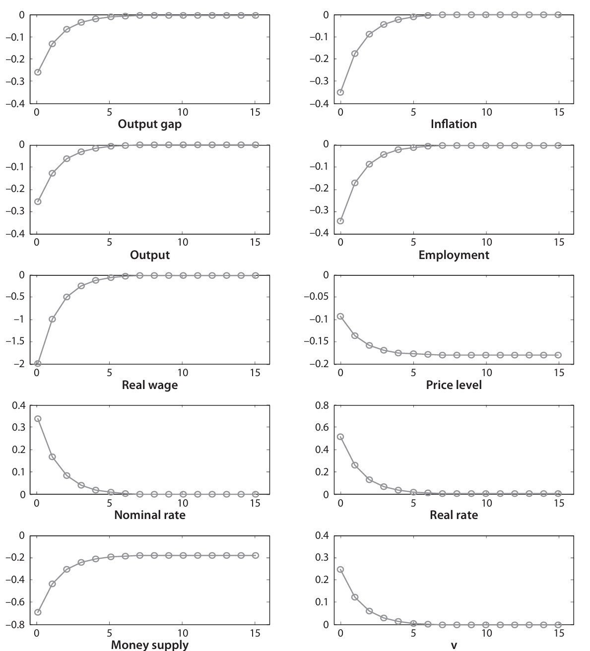
To summarize, calibrated models with non-separable real balances exhibits quantitatively small non-neutralities, large effects of monetary policy shocks on prices, and absence of liquidity effect. An example of non-separability is provided by Walsh (2017). The author specifies a nonseparable utility function, calibrates the model and provides some impulse-response functions to a positive money growth rate shock.

Expansionary monetary policy raises the nominal interest rate — consistently with earlier predictions: higher inflation expectations raise the nominal interest rate. Such an increase contracts labor supply and induces a recession, with lower output and employment. Inflation increases significantly: a 1% shock induces a 2-3% increase in inflation. The real money supply goes down as a result. The unpleasant result is that this model has no liquidity effect: a positive increase in money growth is associated with a positive increase in interest, which is not there in the data. Inflation responds basically immediately, which is also false in the data. An increase in the money supply induces a recession, false in the real world. Finally, and devastatingly, the non-neutrality is tiny: an increase in 1% money growth rate, which leads to a substantial increase in the interest rate, leads to a reduction in output of 0.0something percent, not even captured by the statistical agencies. With non-separable real balances calibrated consistently with empirical estimates of money demand, non-neutralities are very small compared to empirical evidence. This led the literature to cast aside these models for practical purposes.

Alternative Micro-foundations for Money Demand

There are alternative ways to generate demand for money.

• Shopping time models micro-found the demand for money, since leisure is equal to 1 (time endowed) minus the time spent at work and the time that is required to shop: $V(C_t,1-N_t-N_t^s)$. This depends on the shopping technology $N_t^s=S(C_t,L_t)$: real balances facilitate the transactions. Thus, holding real balances increases utility by diminishing the time waste: $U(C_t,N_t,L_t)\equiv V(C_t,1-N_t-S(C_t,L_t))$.
• Cash in advance constraints induce demand for money by introducing an additional constraint: consumption expenditures cannot be larger than the amount of money carried over from the previous perdiod (and cash government transfers): $P_t{C}_t\le M_t+P_t{T}_t$.
• Cash vs credit goods, a generalization by Lucas of cash in advance constraints. Suppose Good 1 is a cash good and Good 2 is a credit good: the latter works like consumption so far (no cash in advance is needed, labor income can be directly transformed in consumption), but cash is needed in advance for Good 1. Interesting implications include that changes in inflation effectively affect the relative price of the two goods, distorcing the quantities consumed in an inefficient way (for further treatment, see PS1).

Global Equilibrium Dynamics

In this section, we will briefly consider equilibria further away from the steady state. In such contexts, log-linearization can no longer be used. Consider an economy like the previous one, with $R=\frac{1}{\beta }$. Money market clearing implies that $\frac{M}{P_t}=YL(Q_t)$ where $L^{\prime }(Q_t)>0$. Assuming perfect foresight and using the relationship between $Q_t$ and inflation, that is $Q_t=\frac{1}{R}\frac{P_t}{P_{t+1}}$ or in logs $i_t=\rho +{\pi }_t$, this becomes $\frac{M}{Y}=P_{t}L\left(\frac{\beta P_t}{P_{t+1}}\right)$. To continue, find consistent steady state paths without linear approximations. A steady state with a constant price level is defined as $P^{\ast }=\frac{M}{YL(\beta )}$. Deviations from this can be found by solving for $P_{t+1}$, with the global equilibrium dynamic: $P_{t+1}=\frac{\beta P_t}{L^{-1}\frac{M}{Y{P}_t}}\equiv \varphi (P_t)$. It is possible to verify that ${\varphi }^{\prime }(P_t)>0$ and ${\varphi }^{\prime }(P^{\ast })>1$. Note that the transversality condition is violated if the dynamics tend to 0 and in particular if ${\lim }_{T\to \infty }\frac{M}{P_T}>0$, since $P_t$ is decreasing at a rate $\beta$ and converging to a positive constant. Thus, it is not an equilibrium. In constrast, equilibria at the right of $P^{\ast }$ cannot be ruled out in general: thus, hyperinflationary equilibria can be, in principle, admitted. This may hold true even if the money supply is constant: in such cases, the steady state is referred to as a self fulfilling hyperinflation, since individuals believe that inflation is incrasing, leading to higher interest rates and lower demand for money, so as to increase the price level. It turns out, however (see Obstfeld and Rogoff, 1983), that these explosive equilibria can be ruled out with a single condition, known as the Obstfeld Rogoff condition: ${\lim }_{L\to 0}L\cdot U_l>0$ which is easily satisfied (even with log-utility). An interpretation consistent with the Walsh figure is that, for a finite $P_t$, then $P_{t+1}$ becomes basically vertical, so that no finite price level is consistent with the equilibrium.

The Fiscal Theory of the Price Level

An unorthodox monetary theory about price determination is the fiscal theory of the price level. In this case, monetary policy is passive, but fiscal policy determines nominal variables. Thus, $Q_t$ is exogenous (constant), there is an exogenous gross constant real interest rate $R_t\equiv \frac{1}{Q_t}\frac{P_t}{P_{t+1}}={\beta }^{-1}$, and assume perfect foresight for simplicity. The period government budget constraint is:

$$\begin{array}{rl}\frac{B_{t-1}^G+M_{t-1}}{P_t}& =Q_t\frac{P_{t+1}}{P_t}\frac{B_t^G+M_t}{P_{t+1}}+(1-Q_t)\frac{M_t}{P_t}+T_t-G_t\\ & =\beta \left(\frac{B_t^G+M_t}{P_{t+1}}\right)+S_t\end{array}$$

where $S_t$ denotes the primary surplus. Note that the government exerts seignorage of size $(1-Q_t)\frac{M_t}{P_t}$. By forward iteration:

$$\begin{array}{rl}\frac{B_{t-1}^G+M_{t-1}}{P_t}& =\sum _{k=0}^{\infty }{\beta }^k{S}_{t+k}+\underset{T\to \infty }{\lim }{\beta }^T\left(\frac{B_{t+T}^G+M_{t+T}}{P_{t+1+T}}\right)\\ \frac{B_{t-1}^G+M_{t-1}}{P_t}& =\sum _{k=0}^{\infty }{\beta }^k{S}_{t+k}\end{array}\text{\hspace{1em}(G-IBC)}$$

were we exploited the transversality condition (solvency constraint combined with optimality). For any exogenous $S_t$, the government’s intertemporal budget constraint (G-IBC) uniquely determines $P_t$. Take an example of passive fiscal policy, that is for a $\Phi >0$:

$$\begin{array}{rl}{S}_t& =\Phi \frac{B_{t-1}^G+M_{t-1}}{P_t}\\ ⟹& \frac{B_t^G+M_t}{P_{t+1}}=\sum _{k=0}^{\infty }{\beta }^k\Phi S_{t+k}=\frac{1-\Phi }{\beta }\frac{B_{t-1}^G+M_{t-1}}{P_t}\\ ⟹& \frac{B_{t+T}^G+M_{t+T}}{P_{t+1+T}}={\left(\frac{1-\Phi }{\beta }\right)}^T\frac{B_{t-1}^G+M_{t-1}}{P_t}\\ ⟹& \underset{T\to \infty }{\lim }{\beta }^T\left(\frac{B_{t+T}^G+M_{t+T}}{P_{t+1+T}}\right)=(1-\Phi {)}^T\frac{B_{t-1}^G+M_{t-1}}{P_t}=0\end{array}$$

The Classical Model and Empirical Evidence

In previous years, the ECB initially adopted the “monetary pillar” for monetary policy, that is it targeted some reference value in the growth of M3 at around to 4.5%, with the aim to pin down inflation anchoring money growth. Despite evidence suggesting that money growth transmits on inflation, it is however not possible to pin down inflation uniquely by controlling the money supply. The Classical model shows that other policy rules, like interest rate rules, can control inflation better than money supply, as the latter can react to many shocks such as money demand shocks. Although it holds in equilibrium that money supply and inflation are related, this is not a direct connection that should be leveraged upon, especially off-equilibrium.

As regards the short run, some predictions of the classical model are too strong and rebuted by the data. Consider the effects of exogenous monetary policy shocks, that is a policy which is not elicited by the economy but imposed exogenously. The paper considered is Christiano, Eichenbaum and Evans (1999), focusing on the federal funds rate — the U.S. main instrument for monetary policy. Suppose for practical purposes that the data generating process for the nominal rate follows a linear model: $i_t=X_t^{⊺}\beta +{\epsilon }_t^m$. Obviously, the errors are not directly observable and have to be measured. A natural approach is estimating the rule and then recovering the residuals; finally, take variables of interest $X_t$ and regress these on the value of current monetary policy shocks, as $X_t={\sum }_{k=0}^{\infty }{\gamma }_k^{⊺}{\epsilon }_{t-1}^m$. This allows to isolate the effect of monetary policy shocks from other shocks. Performing this calculation shows that, when the Federal Funds are raised persistently (persistent tightening), GDP also declines persistently. Second, in the short run, the GDP deflator hardly changes and declines eventually more slowly. Finally, the measure of money supply declines persistently. The key takehome message is that the response of the price level is basically unresponsive of the Funds rate. Moreover, the Classical model predicted no liquidity effect (oney supply and interest rate moved in same direction). Empirically, the opposite occurs: money supply and interest rates move in opposite directions.

Liquidity Effect

Liquidity effect refers to the money supply and the interest rate moving in opposite directions.

Similar results are obtained by Jaroncinski and Karadi (2020), focusing on the 30-minute window span when the Fed announced rates.

Sticky Prices: Evidence, Microfoundations, and Early Models

Microeconomic evidence can help in grounding the patterns followed by individual prices. In particular, it is observed that there are some goods (manufacturing goods, both durables and nondurables, and services) whose prices remain constant for significant amounts of time, and occasionally change discretely in some direction. In contrast, prices for food and energy change more frequently, almost continuously in some cases. In what follows, then, we will focus accordingly on sticky prices. Stickiness refers to the frequency of price changes: the fraction of firms that adjusts the price of individual goos (or the fraction of goods whose price is adjusted in a given month). Empirical evidence suggests that only 12% of prices are adjusted every given month! Moreover, prices in the EU are in general more flexible than the US. Some literature (including Benigno) suggests that more emphasis should be put on stickier prices, and when these start adjusting more frequently, triggering serious inflation spirals. However, only recently did we start collecting data on price changes, and for most of the time inflation was very flat (this changed with the COVID inflation surge). Nakamura, Steinsson, Sun and Villar (QJE, 2020) still tried to reconstruct price adjustment back to the 70s, and realized that the frequency of price change correlates almost by 0 when inflation is low; however, when inflation is triggered, there is a significant positive correlation. This was confirmed in a ECB Economic Bulletin (Dedola et al. 3/2024), while price decreases are absolutely constant and low. Additional evidence in Argentina suggests that low inflation does not affect the frequency of price changes, but when inflation increases then it basically induces more frequent adjustments. Eventually, models of price stickiness assume that the frequency of price changes is constant. However, this is a reasonable simplification only to the extent that inflation remains low and steady. To model episodes of higher inflation, then the sticky prices models would not be appropriate.

Microfoundations for Price Stickiness

In the 80s, microfounding macroeconomics was popularized as a key issue and the main priority. Price stickiness is no less microfounded, as will be showed in this section. Let us consider a firm that sets prices independently, moving away from the assumption of perfect competition. Suppose their profit function is given by $D(p(i),Y)$, where $p(i)\equiv \frac{P(i)}{P}$ and $Y$ is a profit shifter. Real profits for firm $i$ depends on the relative price of the good, and $Y$ shifts the profit function, interpreted as aggregate output. Standard neoclassical assumptions include concavity with respect to prices, that is $D_{pp}<0,D_{py}\ge 0$. The optimal price setting condition requires that: $D_p(p(i{)}^{\ast },Y)=0$ while the optimal price adjustment in response to $dY$ is as follows:$D_{pp}dp(i{)}^{\ast }+D_{py}dY=0$which implies, by multiplying and dividing by the level of $Y$:

$$\begin{array}{rl}dp(i{)}^{\ast }& =-\frac{D_{py}}{D_{pp}}dY\\ & =\Phi dy\end{array}$$

where $\Phi \equiv -Y\frac{D_{py}}{D_{pp}}>0$ is an inverse index of real rigidities. Put simply, if $\Phi$ is large, real rigidities are small; if $\Phi$ are small, there are large real rigidities. Let us consider the economy as a whole, with many identical firms in a symmetric equilibrium. Relative prices must sum up to 1, which induces the initial equilibrium as a symmetric equilibrium with flexible prices $D_p(1,Y_0)=0$, which pins down $Y_0$. A small change in the profit shifter induces a new optimal price $D_p(p(i{)}^{\ast },Y)=0$ when other firms do not adjust, for any reason. $Y$ has not changed, but relative prices are affected. Approximating $D(1,Y)$ near the optimum when firms do not adjust:

$$\begin{array}{rl}D(1,Y)& \approx D(p(i{)}^{\ast },Y)+\stackrel{=0\text{ by optimality}}{\overbrace{D_p(p(i{)}^{\ast },Y)}}(1-p(i{)}^{\ast })+\frac{1}{2}{D}_{pp}(p(i{)}^{\ast },Y)(1-p(i{)}^{\ast }{)}^2\\ & \approx D(p(i{)}^{\ast },Y)+\frac{1}{2}{D}_{pp}(p(i{)}^{\ast },Y)(1-p(i{)}^{\ast }{)}^2\end{array}$$

Thus, the gain from price adjustment when other firms do not adjust is equal to

$$D(p(i{)}^{\ast },Y)-D(1-Y)\approx -\frac{1}{2}{D}_{pp}{\Phi }^2(dy{)}^2>0$$

If we assume that $PY=M$, then $dy+\pi =dm$; since other firms do not adjust, $\pi =0$ and thus $dy=dm$. Rewrite the previous as

$$D(p(i{)}^{\ast },Y)-D(1-Y)\approx -\frac{1}{2}{D}_{pp}{\Phi }^2(dm{)}^2>0$$

that can be also interpreted as the opportunity cost of not adjusting the price. The effects on profits are of second order, normally smaller the flatter the profit function is. The stronger the real rigidities, the smaller the $\Phi$ and thus the smaller the potential profit gain.

However, suppose there is a menu cost, a small cost of adjusting the price. This menu cost may be small, but still larger than the losses for not adjusting the prices. In such cases, firms choose not to adjust the price, and this is an equilibrium. In such cases, inflation is 0 and output changes in proportion to the money supply: the change in money supply has first order real effects. This is more likely to happen for small $\Phi$, weak concavity of the profit function, and the smaller the shock $dm$. If the marginal product of labor is higher than the marginal rate of substitution, as it normally is (due to market power, distortionary taxation, and other practices that make the level of economic activity lower than efficiency), then the economic outcome of increasing money supply has first order welfare effects (that is, effect of the same effect of the change in money supply). The salient result is that tiny, second order menu costs are sufficient to induce first order real effects of monetary shocks.

Multiple equilibria may arise if other firms adjust, and firm $i$ does not adjust its profits. Then, these are given by $D\left(\frac{1}{1+dm},Y\right)$. Approximating around $D(1,Y)$:

$$\begin{array}{rl}D\left(\frac{1}{1+dm},Y\right)& \approx D(1,Y)+D_p(1,Y)\left(\frac{1}{1+dm}-1\right)+\frac{1}{2}{D}_{pp}(1,Y){\left(\frac{1}{1+dm}-1\right)}^2\\ & \approx D(1,Y)+\frac{1}{2}{D}_{pp}{\left(\frac{dm}{1+dm}\right)}^2\end{array}$$

Which implies a gain from price adjustment when other firms adjust equal to

$$D(1,Y)-D\left(\frac{1}{1+dm},Y\right)\approx -\frac{1}{2}{D}_{pp}{\left(\frac{dm}{1+dm}\right)}^2>0$$

Note that multiple equilibria may occur if the following condition holds: $D(1,Y)-D\left(\frac{1}{1+dm},Y\right)>\varkappa >D(p(i{)}^{\ast },Y)-D(1,Y)$or equivalently $\Phi <\frac{1}{1+dm}$.

A Model with Price-Setting Advantage

The classical reference for this is Blanchard and Kiyotaki (1987), although we’ll consider Romer’s (2019) version. Consider the usual infinitely-lived utility maximizing households with objective function $\max {\mathbb{E}}_0{\sum }_{t=0}^{\infty }{\beta }^{t}U(C_t,N_t)$, where $C_t={\left({\int }_0^1{C}_t(i{)}^{1-1/\epsilon }di\right)}^{\frac{ϵ}{ϵ-1}}$. That is, $C_t$ is an index of the quantity of good consumed for a continuum of goods $i$, where the CES function suggests that goods have some degree of substitution elasticity $ϵ>1$. As usual $\beta \equiv e^{-\rho }$. The usual resource constraint and cash-in-advance constraint hold:

$$\{\begin{array}{l}{\int }_0^1{P}_t(i)C_t(i)di+Q_t{B}_t+M_t\le B_{t-1}+M_{t-1}+P_t{D}_t-P_t{T}_t\\ {\int }_0^1{P}_t(i)C_t(i)di+P_t{T}_t\le M_{t-1}\end{array}$$

together with the usual solvency constraint

$$\underset{T\to \infty }{\lim }{\mathbb{E}}_t\{{\Lambda }_{t,t+T},{\mathcal{A}}_{t+T}\}\ge 0$$

where ${\mathcal{A}}_t\equiv \frac{B_{t-1}+M_{t-1}}{P_t}$

The important feature of the model is that firms set prices before economic shocks occur, and once these happen firms are stuck to their prices for one period. This one period delay is the main source of price stickiness. Last, money demand will be introduced as a cash-in-advance constraint. This and the budget constraint appear as in the classical model, with the only difference in the consumption integral.

Household optimality

In a first stage, solve the problem of optimal allocation of expenditure. For every given consumption index, it is optimal for the households to minimize the expenditure in order to obtain such level of consumption for each specific commodity, subject to attaining the level of final consumption index $C_t$: that is

$$\underset{\{C_t(i)\}}{\min }{\int }_0^1{P}_t(i)C_t(i)di\text{such that }{\left({\int }_0^1{C}_t(i{)}^{1-\frac{1}{ϵ}}di\right)}^{\frac{ϵ}{ϵ-1}}=C_t$$

It can be shown that the optimality condition is satisfied given the following implied demand function for each good:

$$C_t(i)={\left(\frac{P_t(i)}{P_t}\right)}^{-ϵ}{C}_t$$

where $P_t={\left({\int }_0^1{P}_t(i{)}^{1-ϵ}di\right)}^{\frac{1}{1-ϵ}}$. The additional implication is that the implied demand function satisfies the following condition, so as to be written conveniently as

$${\int }_0^1{P}_t(i)C_t(i)di=P_t{C}_t$$

allowing to tread the problem as if there were a single good.

Price Level

The aggregate price level $P_t$ is defined as:

$$P_t:={\left({\int }_0^1{P}_t(j{)}^{1-ϵ}dj\right)}^{\frac{1}{1-ϵ}}$$

Raising both sides to the power of $1-ϵ$:

$$P_t^{1-ϵ}={\int }_0^1{P}_t(j{)}^{1-ϵ}dj$$

Substituting this back into the expression for $C_t$:

$$C_t(i)P_t(i{)}^{ϵ}{\left(P_t^{1-ϵ}\right)}^{\frac{ϵ}{ϵ-1}}=C_t(i)P_t(i{)}^{ϵ}{P}_t^{-ϵ}$$

In a second stage, determine optimal consumption, money supply and labor demand. This is the same problem solved in the classical model, with the additional assumption that the nominal interest rate is positive (in equilibrium) and thus the cash in advance constraint will always be satisfied with equality. Set up the Lagrangian:

$$\mathcal{L}={\int }_0^1{P}_t(i)C_t(i)di+\lambda \left[C_t-{\left({\int }_0^1{C}_t(i{)}^{1-1/ϵ}di\right)}^{\frac{ϵ}{ϵ-1}}\right]$$

with FOC:

$$\begin{array}{rl}\frac{\partial \mathcal{L}}{\partial C_t(i)}& =0\\ \frac{\partial }{\partial C_t(i)}{\int }_0^1{P}_t(i)C_t(i)di& =-\lambda \frac{\partial }{\partial C_t(i)}{\left({\int }_0^1{C}_t(i{)}^{1-1/ϵ}di\right)}^{\frac{ϵ}{ϵ-1}}\\ {\int }_0^1\frac{\partial }{\partial C_t(i)}{P}_t(i)C_t(i)di& =-\frac{ϵ}{ϵ-1}\lambda {\left({\int }_0^1{C}_t(i{)}^{1-1/ϵ}di\right)}^{\frac{1}{ϵ-1}}\frac{\partial }{\partial C_t(i)}{\int }_0^1{C}_t(s{)}^{1-1/ϵ}ds\\ {\int }_0^1\frac{\partial }{\partial C_t(i)}{P}_t(i)C_t(i)di& =-\frac{ϵ}{ϵ-1}\lambda {\left({\int }_0^1{C}_t(i{)}^{1-1/ϵ}di\right)}^{\frac{1}{ϵ-1}}{\int }_0^1\frac{\partial C_t(i{)}^{\frac{ϵ-1}{ϵ}}}{\partial C_t(i)}\frac{\partial C_t(i)}{\partial C_t(s)}ds\\ {\int }_0^1\frac{\partial }{\partial C_t(i)}{P}_t(i)C_t(i)di& =-\frac{ϵ}{ϵ-1}\lambda {\left({\int }_0^1{C}_t(i{)}^{1-1/ϵ}di\right)}^{\frac{1}{ϵ-1}}{\int }_0^1\frac{\partial C_t(i{)}^{\frac{ϵ-1}{ϵ}}}{\partial C_t(i)}\delta (s-i)ds\\ P_t(i)& =\frac{ϵ}{ϵ-1}\lambda {\left({\int }_0^1{C}_t(i{)}^{1/ϵ}di\right)}^{\frac{1}{ϵ-1}}\frac{ϵ-1}{ϵ}{C}_t(i{)}^{-\frac{1}{ϵ}}\\ P_t(i)& =\lambda {\left({\int }_0^1{C}_t(i{)}^{1/ϵ}di\right)}^{\frac{1}{ϵ-1}}{C}_t(i{)}^{-\frac{1}{ϵ}}\end{array}$$

which holds for all $i\in [0,1]$ (the derivative has been derived exploiting the property of the Dirac Delta, here denoted as $\delta$, of integrating to 1). Note that:

$$\{\begin{array}{ll}{C}_t(i)& ={\left(\frac{P_t(i)}{\lambda {\left({\int }_0^1{C}_t(i{)}^{1/ϵ}di\right)}^{\frac{1}{ϵ-1}}}\right)}^{-ϵ}\\ C_t(j)& ={\left(\frac{P_t(j)}{\lambda {\left({\int }_0^1{C}_t(i{)}^{1/ϵ}di\right)}^{\frac{1}{ϵ-1}}}\right)}^{-ϵ}\end{array}⟹C_t(j)={\left(\frac{P_t(i)}{P_t(j)}\right)}^{ϵ}{C}_t(i)$$

which allows to compute the aggregate demand for consumption goods:

$$\begin{array}{rl}{C}_t& :={\left({\int }_0^1{C}_t(j{)}^{\frac{ϵ-1}{ϵ}}dj\right)}^{\frac{ϵ}{ϵ-1}}\\ & ={\left({\int }_0^1{\left[{\left(\frac{P_t(i)}{P_t(j)}\right)}^{ϵ}{C}_t(i)\right]}^{\frac{ϵ-1}{ϵ}}dj\right)}^{\frac{ϵ}{ϵ-1}}\\ & =C_t(i)P_t(i{)}^{ϵ}{\left({\int }_0^1{P}_t(j{)}^{1-ϵ}dj\right)}^{\frac{ϵ}{ϵ-1}}\\ & =C_t(i)P_t(i{)}^{ϵ}{P}_t^{-ϵ}\\ ⟺C_t(i)& ={\left(\frac{P_t(i)}{P_t}\right)}^{-ϵ}{C}_t\end{array}$$

Recall that the households optimality conditions are as follows:

$$\begin{array}{rl}-\frac{U_{n,t}}{U_{c,t}}& =\frac{W_t}{P_t}\\ Q_t& =\beta \mathbb{E}\left[\frac{U_{c,t+1}}{U_{c,t}}\frac{P_t}{P_{t+1}}\right]\\ P_t{C}_t+P_t{T}_t& =M_{t-1}\end{array}$$

Moreover, it can be assumed in equilibrium that $P_t{T}_t=-\Delta M_t$, and thus $P_t{C}_t=M_t$. Assume the conventional CRRA utility function and derive the log-linearized optimality conditions:

$$\begin{array}{rl}U(C_t,N_t)& =\{\begin{array}{ll}\frac{C_t^{1-\sigma }-1}{1-\sigma }-\frac{N_t^{1+\varphi }}{1+\varphi }& \sigma \ne 1\\ \log (C_t)-\frac{N_t^{1+\varphi }}{1+\varphi }& \sigma =1\end{array}\\ & \\ w_t-p_t& =\sigma c_t+\varphi n_t\\ c_t& =\mathbb{E}[c_{t+1}]-\frac{1}{\sigma }(i_t-\mathbb{E}[{\pi }_{t+1}]-\rho )\\ m_t& =p_t+c_t\end{array}$$

Firm optimality: Flexible prices

The firm problem changes as the firm can set the price, subject to a demand constraint (monopolistic competition). As will be shown below, the optimality condition is equal to the desired markup $\mathcal{M}\equiv \frac{ϵ}{ϵ-1}$ times the production cost given the output. To set up the problem, consider the usual technology $Y_t(i)=A_t{N}_t(i{)}^{1-\alpha }$ and define the (log-linearized) wage-to-marginal-product-of-labor ratio:

$${\psi }_t(i)=w_t-[a_t-\alpha n_t(i)+\log (1-\alpha )]$$

It is now possible to set up the firms’ profit maximization problem subject to the cost function $\mathcal{C}$:

$${\varpi }_t:=\underset{P_t(i)}{\max }{P}_t(i)Y_t(i)-\mathcal{C}(Y_t(i))\text{subject to }{Y}_t(i)={\left(\frac{P_t(i)}{P_t}\right)}^{-ϵ}{C}_t$$

as previously derived. To obtain the optimality conditions, take the derivative of the objective function with respect to $P_t(i)$, equate it to 0, and then produce the quantity determined by the demand function by imposing the constraint:

$$\begin{array}{rl}\frac{\partial \varpi }{\partial P_t(i)}& =0\\ \frac{\partial }{\partial P_t(i)}[P_t(i)Y_t(i)-\mathcal{C}(Y_t(i))]& =0\\ \frac{\partial }{\partial P_t(i)}\left[P_t(i{)}^{1-ϵ}{P}_t^{ϵ}{C}_t-\mathcal{C}\left({\left(\frac{P_t(i)}{P_t}\right)}^{-ϵ}{C}_t\right)\right]& =0\\ (ϵ-1)P_t(i{)}^{-ϵ}{P}_t^{ϵ}{C}_t& =ϵP_t(i{)}^{-ϵ-1}{P}_t^{ϵ}{C}_t{\Psi }_t(i)\\ P_t(i{)}^{-ϵ}& =\frac{ϵ}{ϵ-1}{P}_t(i{)}^{-ϵ-1}{\Psi }_t(i)\end{array}$$

which leads to:

$$P_t(i)={\mathcal{M}}_t{\Psi }_t(i)$$

Two new objects are hereby introduced:

• the desired markup ${\mathcal{M}}_t(i)\equiv \frac{ϵ}{ϵ-1}$
• the marginal cost of labor ${\Psi }_t(i)\equiv {\mathcal{C}}^{\prime }(Y_t(i))$, which is firm-specific as different production level may induce different marginal costs. Note that the previous result implies that the desired markup is constant and equal to

$$\mathcal{M}\equiv \frac{P_t(i)}{{\Psi }_t(i)}={\mathcal{M}}_t(i)$$

The optimality condition of the firm can be log-linearized, and extended to the aggregate firm sector invoking symmetry:

$$\begin{array}{rl}{p}_t(i)& =\mu +{\psi }_t(i)\\ p_t& =\mu +{\psi }_t\end{array}$$

which compares to the perfect competition scenario as:

$$w_t-p_t=mp{n}_t⟹p_t=w_t-mp{n}_t={\psi }_t$$

To compute the equilibrium, exploit the price setting equation. Recall that, given our production function, the marginal cost is equal to ${\Psi }_t=W_t-(1-\alpha {)}_t{A}_t{N}^{-\alpha }$ which is log-linearized as ${\psi }_t=w_t-a_t+\alpha n_t-\log (1-\alpha )$. This can be seen as follows:

$$\begin{array}{rl}{N}_t& ={\int }_0^1{N}_t(i)di\\ & ={\int }_0^1{\left(\frac{Y_t(i)}{A_t}\right)}^{\frac{1}{1-\alpha }}di\\ & ={\left(\frac{Y_t}{A_t}\right)}^{\frac{1}{1-\alpha }}{\int }_0^1{\left(\frac{P_t(i)}{P_t}\right)}^{-\frac{ϵ}{1-\alpha }}di\\ (1-\alpha )n_t& =y_t-a_t+\log \left\{(1-\alpha ){\int }_0^1{\left(\frac{P_t(i)}{P_t}\right)}^{-\frac{ϵ}{1-\alpha }}\right\}\end{array}$$

where $\log \left\{(1-\alpha ){\int }_0^1{\left(\frac{P_t(i)}{P_t}\right)}^{-\frac{ϵ}{1-\alpha }}\right\}$ is an index of price dispersion and is equal to zero up to a first order approximation (the result is proved below).

Price Dispersion

By definition of $P_t$:

$$1={\int }_0^1{\left(\frac{P_t(i)}{P_t}\right)}^{1-ϵ}di\text{\hspace{1em}(A)}$$

Note that it can be rewritten ${\left(\frac{P_t(i)}{P_t}\right)}^{1-ϵ}=\exp \{(1-ϵ){\hat{p}}_t\}$, where ${\hat{p}}_t=p_{t(i)-p_t}$. Its second order approximation yields:

$$\begin{array}{rl}\exp \{(1-ϵ){\hat{p}}_t\}& \approx 1+(1-ϵ){\hat{p}}_t(i)+\frac{1}{2}(1-ϵ{)}^2{\hat{p}}_t(i)\\ 0& \approx (1-ϵ){\mathbb{E}}_i[{\hat{p}}_t(i)]+\frac{1}{2}{\mathbb{E}}_i[{\hat{p}}_t(i)]\\ {\mathbb{E}}_i[{\hat{p}}_t(i)]& \approx \frac{ϵ-1}{2}{\mathbb{E}}_i[{\hat{p}}_t(i{)}^2]\end{array}$$

This can be plugged in a second-order approximation of ${\left(\frac{P_t(i)}{P_t}\right)}^{-\frac{ϵ}{1-\alpha }}$ around 0, that is $1+\frac{1}{2}{\left(\frac{ϵ}{1-\alpha }\right)}^2{\hat{p}}_t(i)$, so as to obtain:

$$\begin{array}{rl}{\int }_0^1{\left(\frac{P_t(i)}{P_t}\right)}^{-\frac{ϵ}{1-\alpha }}di& =1+\frac{1}{2}\left(\frac{ϵ}{1-\alpha }\right)\frac{1}{\Theta }{\text{var}}_i(p_t(i))\end{array}$$

where $\Theta =\frac{1-\alpha }{1-\alpha +\alpha ϵ}$. Plugging this into the definition of price dispersion, that is equal - up to a second order approximation - to:

$$d_t\approx \frac{ϵ}{2\Theta }{\text{var}}_i(p_t(i))$$

Thus:

$$\begin{array}{rl}{p}_t& =\mu +{\psi }_t\\ & =\mu +w_t-a_t+\alpha n_t-\log (1-\alpha )\\ 0& =\mu +\sigma y_t+\varphi n_t-a_t+\alpha n_t-\log (1-\alpha )\\ 0& =\mu +\sigma a_t+\sigma (1-\alpha )n_t+\varphi n_t-a_t+\alpha n_t-\log (1-\alpha )\\ 0& =n_t[\sigma (1-\alpha )+\varphi +\alpha ]+\mu +\sigma a_t-a_t-\log (1-\alpha )\\ -n_t& =\frac{\mu +(\sigma -1)a_t-\log (1-\alpha )}{\sigma (1-\alpha )+\varphi +\alpha }\\ \frac{a_t-y_t}{1-\alpha }& =\frac{\mu -\log (1-\alpha )}{\sigma (1-\alpha )+\varphi -\alpha }+\frac{a_t(\sigma -1)}{\sigma (1-\alpha )+\varphi -\alpha }\\ -y_t& =\frac{(1-\alpha )[\mu -\log (1-\alpha )]}{\sigma (1-\alpha )+\varphi +\alpha }+a_t\left(\frac{(1-\alpha )(\sigma -1)}{\sigma (1-\alpha )+\varphi +\alpha }-1\right)\\ y_t& =\frac{(1-\alpha )[\log (1-\alpha )-\mu ]}{\sigma (1-\alpha )+\varphi +\alpha }+a_t\frac{1+\varphi }{\sigma (1-\alpha )+\varphi +\alpha }\end{array}$$

where the equalities in line 2, 3, 4 and 5 follow respectively from the definition of ${\psi }_t$, from the household optimality conditions at ^1fa0f4, from market clearing and the technological constraint. Recall the goods market clearing condition $y_t=c_t$, and the production function $y_t=a_t+(1-\alpha )n_t$ which allows to express labor supply as $n_t=\frac{y_t-a_t}{1-\alpha }$. The level of output derived under flexible prices can be referred to as the natural level of output and denoted as $y_t^n$:

$$y_t={\psi }_{ya}{a}_t+{\psi }_y^{\mu }\equiv y_t^n$$

where ${\psi }_{ya}\equiv \frac{1+\varphi }{\sigma (1-\alpha )+\varphi +\alpha }$ and ${\psi }_y^{\mu }\equiv \frac{(1-\alpha )[\log (1-\alpha )-\mu ]}{\sigma (1-\alpha )+\varphi +\alpha }$. Comparing this expression to the classical monetary model case, note that this is almost identical. The only difference lies in the markup, which of course could not be present in the classical model due to perfect competition. Put simply, the fact that firms are monopolistic competitors does not change the way the output responds to technology shocks. The introduction of market power affects only the mean level of output at the steady state: it lowers the level around which output fluctuates, without changing the response to shocks. As for the real interest rate, this remains totally unaffected, with same mean as before.

Employment, real wages, and the real rate

Compute the levels of employment, real wages, and real interest rate and compare these to the classical model. In the flexible prices monopolistic model, these three quantities are as follows:

$$\{\begin{array}{ll}{n}_t& =\frac{\log (1-\alpha )+a(1-\sigma )-\mu }{\sigma (1-\alpha )+\varphi +\alpha }\\ {\omega }_t& =\frac{[\sigma (1-\alpha )+\varphi ][\log (1-\alpha )-\mu ]}{\sigma (1-\alpha )+\varphi +\alpha }+\frac{\sigma +\varphi }{\sigma (1-\alpha )+\varphi +\alpha }{a}_t\\ r_t& =\rho -\sigma {\psi }_{ya}(1-{\rho }_a)a_t+(1-{\rho }_z)z_t\end{array}$$

which compares to the classical model as follows:

$$\{\begin{array}{ll}{n}_t& =\frac{\log (1-\alpha )+a_t(1-\alpha )}{\sigma (1-\alpha )+\varphi +\alpha }\\ {\omega }_t& =\frac{[\sigma (1-\alpha )+\varphi ]\log (1-\alpha )}{\sigma (1-\alpha )+\varphi +\alpha }+\frac{\sigma +\varphi }{\sigma (1-\alpha )+\varphi +\alpha }{a}_t\\ r_t& =\rho -\sigma {\psi }_{ya}(1-{\rho }_a)a_t+(1-{\rho }_z)z_t\end{array}$$

These objects are also referred to as ${\psi }_{ya}\equiv \frac{1+\varphi }{\sigma (1-\alpha )+\varphi +\alpha }$ and ${\psi }_y^{\mu }\equiv \frac{(1-\alpha )[\log (1-\alpha )-\mu ]}{\sigma (1-\alpha )+\varphi +\alpha }$. Note that the main discriminant of the two is the realized markup, shifting the outcome component of the monopolistic model. However, the real rate is the same as in the classical model, since ${\psi }_{ya}$ and $a_t$ are not affected by the markup.

Firm optimality: Nominal rigidities

Now assume that prices are set in advance, that is at the beginning of each period before the shock are realized (sticky prices) rather than at the end of the period in response to just occurred shocks (flexible prices). The new firm problem is as follows:

$$\underset{P_t(i)}{\max }{\mathbb{E}}_{t-1}\left\{{\Lambda }_{t-1,t}\frac{1}{P_t}[P_t(i)Y_t(i)-{\mathcal{C}}_t(Y_t(i))]\right\}\text{subject to }{Y}_t(i)={\left(\frac{P_t(i)}{P_t}\right)}^{-ϵ}{C}_t$$

where ${\Lambda }_{t-1,t}\equiv \beta \frac{U_{c,t}}{U_{c,t-1}}$. The optimality conditions follow a derivation similar to the model with flexible prices and yields:

$${\mathbb{E}}_{t-1}\left\{{\Lambda }_{t-1,t}{Y}_t(i)\frac{1}{P_t}[P_t(i)-\mathcal{M}{\Psi }_t(i)]\right\}=0$$

or, equivalently, by factorizing out ${\Psi }_t(i)$:

$${\mathbb{E}}_{t-1}\left\{{\Lambda }_{t-1,t}{Y}_t(i)\frac{{\Psi }_t(i)}{P_t}[{\mathcal{M}}_t(i)-\mathcal{M}]\right\}=0$$

where ${\mathcal{M}}_t(i)\equiv \frac{P_t(i)}{{\Psi }_t(i)}$. This suggests a perfect foresight steady steady as $\mathcal{M}(i)=\mathcal{M}$.

To log linearize the optimality conditions of the firm, beware not to log-linearize by Taylor expanding around $P_t$ or ${\Psi }_t$: these quantities have ne steady state value, and when they are shocked they move permanently. Instead, in order to transform the conditions into state steady variables, divide and multiply by ${\Psi }_t(i)$, and express everything in terms of the markup. Note that both ${\Psi }_t(i)$ and $P_t(i)$ are equal to 0 when evaluated at the steady state, since these are chosen optimally. Find that the firm will set the price so that the expected markup equalizes the desired markup.

$$\begin{array}{rl}{\mathbb{E}}_{t-1}\left\{{\Lambda }_{t-1,t}{Y}_t(i)\frac{{\Psi }_t(i)}{P_t}[{\mathcal{M}}_t(i)-\mathcal{M}]\right\}& =0\\ \approx {\mathbb{E}}_{t-1}\left\{\left(\overline{\Lambda Y\frac{\Psi }{P}}\right)[{\mathcal{M}}_t(i)-\mathcal{M}]\right\}& \approx 0\\ {\mathbb{E}}_{t-1}\left\{\left(\beta \bar{Y}\overline{\frac{\Psi }{P}}\right)[{\mathcal{M}}_t(i)-\mathcal{M}]\right\}& \approx 0\\ {\mathbb{E}}_{t-1}\left\{[{\mathcal{M}}_t(i)-\mathcal{M}]\right\}& \approx 0\\ \approx {\mathbb{E}}_{t-1}\left\{\log ({\mathcal{M}}_t(i))-\log (\mathcal{M})\right\}& \approx 0\end{array}$$

$$\{\begin{array}{l}{\mathbb{E}}_{t-1}[{\mu }_t(i)]\approx \mu \\ p_t(i)-{\mathbb{E}}_{t-1}[{\psi }_t(i)]=\mu \end{array}$$

where linear approximations have been introduced in the second line and in the sixth line (Jensen’s inequality). A comment on $\frac{{\Psi }_t(i)}{P_t}$: this is the firm’s nominal marginal cost divided by the aggregate price level and represents a form of real marginal cost. In the steady-state, nominal marginal cost tend to grow with the aggregate price level; thus, their ratio is often stationary, even if the element themselves are not. Symmetry can be invoked so as to generalize these conditions:

$$\begin{array}{c}{\mathbb{E}}_{t-1}[{\mu }_t]=\mu \\ p_t=\mu +{\mathbb{E}}_{t-1}[{\psi }_t]\end{array}$$

and finally to compute the average markup in the economy:

$$\begin{array}{rl}{\mu }_t& =p_t-{\psi }_t\\ & =p_t-w_t+a_t-\alpha n_t+\log (1-\alpha )\\ & =-\sigma c_t-\varphi n_t-w_t+a_t-\alpha n_t+\log (1-\alpha )\\ & =-\sigma y_t-\varphi n_t-w_t+a_t-\alpha n_t+\log (1-\alpha )\\ & =-\sigma y_t-n_t(\varphi +\alpha )-w_t+a_t+\log (1-\alpha )\\ & =-\sigma y_t+\left(\frac{a_t-y_t}{1-\alpha }\right)(\varphi +\alpha )-w_t+a_t+\log (1-\alpha )\\ & =-\sigma y_t-\frac{\alpha y_t}{1-\alpha }+\frac{\alpha a_t}{1-\alpha }-\frac{\varphi y_t}{1-\alpha }+\frac{\varphi a_t}{1-\alpha }-a_t+\log (1-\alpha )\\ & \\ {\mu }_t& =-\left(\sigma +\frac{\varphi +\alpha }{1-\alpha }\right)y_t+\left(1+\frac{\varphi +\alpha }{1-\alpha }\right)a_t+\log (1-\alpha )\end{array}$$

Which differs from the flexible prices case simply by the $y_t$, which is $y_t^n={\psi }_{ya}{a}_t+{\psi }_y^{\mu }$ under flexible prices. Put simply, there is a difference between the average markup and the realized markup, which is defined as the output gap ${\tilde{y}}_t\equiv y_t-y_t^n$:

$${\mu }_t-\mu =-\left(\sigma +\frac{\varphi +\alpha }{1-\alpha }\right){\tilde{y}}_t$$

Why does markup decrease in output? This is because increased output induces higher wages, and thus consumption and real wage to the labor supply equilibrium. At the same time, the marginal cost will increase - for the same reason, and also due to decreasing returns to labor ($\alpha >0$). A positive shock to technology increases the markup for any level of output by directly reducing marginal costs. By subtracting the average mark up to output, we obtain the output gap ${\tilde{y}}_t\equiv y_t-y_t^n$. This allows to rewrite the equilibrium condition as a zero output gap condition in expectation.

$$\begin{array}{rl}{\mathbb{E}}_{t-1}[{\tilde{y}}_t]& =0\\ ⟹{\mathbb{E}}_{t-1}[y_t]& ={\mathbb{E}}_{t-1}[y_t^n]\\ & ={\psi }_{ya}{\rho }_a{a}_{t-1}+{\psi }_y^{\mu }\end{array}$$

Output is in equilibrium at:

$$\begin{array}{rl}{y}_t& ={\mathbb{E}}_{t-1}[y_t]+(y_t-{\mathbb{E}}_{t-1}[y_t])\\ & ={\mathbb{E}}_{t-1}[y_t^n]+{\xi }_t^y\\ & ={\psi }_{ya}{\rho }_a{a}_{t-1}+{\psi }_y^{\mu }+{\xi }_t^y\end{array}$$

where ${\xi }_t^y=y_t-{\mathbb{E}}_{t-1}[y_t]$ is “innovation” in output. This equilibrium condition can be used to determine output, prices, and other variables. If gap is 0, the expected output attains its natural level (in expectation). This can be determined by its (expected) equation (it is always possible to write down the realized level of output as the sum of the expectation plus to the “surprise” or innovation, as a sort of forecast error). In the resulting equilibrium, price level is predetermined:

$$\begin{array}{rl}{p}_t& ={\mathbb{E}}_{t-1}[m_t]-{\mathbb{E}}_{t-1}[y_t]\\ & ={\mathbb{E}}_{t-1}[m_t]-{\psi }_{ya}{\rho }_a{a}_{t-1}-{\psi }_y^{\mu }\end{array}$$

In open contrast to the classical model, monetary policy is not neutral through its unanticipated component ${\xi }_t^m$, which affects output. This non-neutrality has two dimensions: on the exogenous end, monetary policy shock affects output (${ϵ}_t^m$); as for the endogenous component, monetary policy will also an effect of output, by the affecting choice of ${\varphi }_a$ (defining such parameter is like allowing for the central bank to react to technology shocks systematically). This is part of the endogenous component of the rule of monetary policy. Therefore, technology shocks affect output in two ways: through monetary policy, and by the marginal cost, but in lag ${\psi }_{ya}{\rho }_a{a}_{t-1}$. To see this, consider a money supply rule such as

$$m_t={\varphi }_z{z}_{t-1}+{\varphi }_a{ϵ}_t^a+{ϵ}_t^m$$

such that ${\xi }_t^m={\varphi }_a{ϵ}_t^a+{ϵ}_t^m$. The output gap is affected by the exogenous monetary shock:

$$\begin{array}{rl}{y}_t& ={\psi }_t^{\mu }+{\psi }_{ya}{\rho }_a{a}_{t-1}+{\varphi }_a{ϵ}_t^a+{ϵ}_t^m\\ {\tilde{y}}_t& ={\psi }_t^{\mu }+{\psi }_{ya}{\rho }_a{a}_{t-1}+{\varphi }_a{ϵ}_t^a+{ϵ}_t^m-{\psi }_{ya}{a}_t-{\psi }_y^{\mu }\\ & =({\varphi }_a-{\psi }_{ya}){ϵ}_t^a+{ϵ}_t^m\end{array}$$

In this model, monetary policy is no longer neutral, finally accommodating empirical evidence. However, it is not such in a very trivial way: monetary shocks only have contemporaneous effects and no persistent effects on output. However, data suggest that the effect of monetary shocks on output is persistent. Since price stickyness has been introduced as lasting for one period only, monetary policy cannot be persistent, as it goes back to the flexible prices results after only one period (other shocks being absent). Another limitation of this model is that inflation has no welfare costs, due to the fact that there are no relative price distortions (all firms adjust samely). In what follows, we’ll consider a model with staggered price setting: at each point in time, only a fraction of firms will adjust prices.

Last, note that with sticky prices the Friedman rule does not hold. The central bank can influence output, and thus will attempt to make the outcome as close as possible as the flexible price equilibrium. This can be done by choosing a rule with ${\varphi }_a={\psi }_{ya}$, and no monetary policy shocks as these would cancel out. That would be the optimal policy in such scenario. In that case, the output gap would always be at 0, and the would replicate the flexible price equilibrium. However, it is no longer an efficient equilibrium due to the monopolistic competition assumption.

The Basic New Keynesian Model

This section will introduce price staggering, referring to a pricing environment where only a random fraction of firms adjusts prices at every period. This is motivated by the microeconomic evidence previously discussed. As for the rest, continue assuming competitive markets. The New Keynesian model, derived from the previous assumption, is sometimes referred to as the Three-Equation model since it is indeed described by three equations:

$$\{\begin{array}{ll}{\pi }_t& =\beta {\mathbb{E}}_t[{\pi }_{t+1}]+\kappa {\tilde{y}}_t\\ {\tilde{y}}_t& =-\frac{1}{\sigma }(i_t-{\mathbb{E}}_t[{\pi }_{t+1}]-r_t^n)+{\mathbb{E}}_t[{\tilde{y}}_{y+1}]\\ i_t& =\rho +{\varphi }_{\pi }{\pi }_t+{\varphi }_y{\hat{y}}_t+v_t\end{array}$$

These are referred to as the New Keynesian Phillips Curve, Dynamics IS Equation, and Monetary Policy Rule respectively. The policy rule can vary depending on the model specifications.

In this model, it will be explained that the identity between realized and desired markups holds only in the zero inflation steady state, not in every steady state. Whenever the firms markup is, on average too low relative to desired markup, they will steadily increase prices when given the opportunity to do so, but they will be able to do so only occasionally. Inflation will thus be driven by the tension between the realized and desired markup.

Household preferences and budget constraint are the same as before (without the cash-in-advance constraint), with optimality conditions:

$$\{\begin{array}{l}-\frac{U_{n,t}}{U_{c,t}}=\frac{W_t}{P_t}\\ Q_t=\beta {\mathbb{E}}_t\left[\frac{U_{c,t+1}}{U_{c,t}}\frac{P_t}{P_{t+1}}\right]\end{array}$$

In addition to the optimal allocation of expenditure, compute the optimal consumption, labor supply, and money demand, based on the usual optimality conditions as derived in the classical model. We add an exogenous preference shock to the utility function of the households, modeled as an exogenous stochastic process $z_t\equiv \log Z_t$ such that $z_t={\rho }_z{z}_{t-1}+{ϵ}_t^z$, and a money demand shifter ${\Xi }_t\equiv e^{{\xi }_t}$:

$$U(C_t,N_t)=\{\begin{array}{ll}\left(\frac{C_t^{1-\sigma }-1}{1-\sigma }-\frac{N_t^{1+\varphi }}{1+\varphi }+{\Xi }_t^{\sigma }\frac{L_t^{1-\sigma }-1}{1-\sigma }\right)Z_t& \sigma \ne 1\\ \left(\log (C_t)-\frac{N_t^{1+\varphi }}{1+\varphi }+{\Xi }_t^{\sigma }\log (L_t)\right)Z_t& \sigma =1\end{array}$$

Note that the assumption of separable real balances is still in place, ruling out any impact of $L$ on $-\frac{U_{n,t}}{U_{c,t}}$. Finally, given the CRRA specification that is chosen, these optimality conditions can expressed explicitly as:

$$\{\begin{array}{ll}{U}_{c,t}& =C_t^{-\sigma }{Z}_t\\ -U_{n,t}& =N_t^{\varphi }{Z}_t\\ U_{l,t}& ={\Xi }_t^{\sigma }{L}_t^{-\sigma }{Z}_t\end{array}$$

leading to the implied optimality conditions:

$$\{\begin{array}{ll}\frac{W_t}{P_t}& =C_t^{\sigma }{N}_t^{\varphi }\\ Q_t& =\beta {\mathbb{E}}_t\left[{\left(\frac{C_{t+1}}{C_t}\right)}^{-\sigma }\frac{Z_{t+1}}{Z_t}\frac{P_t}{P_{t+1}}\right]\\ L_t& =C_t(1-e^{-i_t}{)}^{-\frac{1}{\sigma }}{\Xi }_t\end{array}$$

and their log-linear counterparts:

$$\{\begin{array}{l}{w}_t-p_t=\sigma c_t+\varphi n_t\\ c_t={\mathbb{E}}_t[c_{t+1}]-\frac{1}{\sigma }(i_t-{\mathbb{E}}_t[{\pi }_{t+1}]-\rho )+\frac{1}{\sigma }(1-{\rho }_z)z_t\end{array}$$

where the second condition can be derived by taking a first order approximation around a steady state with constant growth and inflation, recalling that in such steady state $i=\rho +\pi +\sigma y$, and rewriting the consumer’s Euler equation as $1={\mathbb{E}}_t[\exp \{i_t-\sigma \Delta c_{t+1}-{\pi }_{t+1}-\rho +\Delta x_{t+1}\}]$:

$$\begin{array}{rl}1& ={\mathbb{E}}_t[\exp [i_t-\sigma \Delta c_{t+1}-{\pi }_{t+1}-\rho +\Delta x_{t+1}]]\\ & \approx {\mathbb{E}}_t[1+i_t-\sigma \Delta c_{t+1}-{\pi }_{t+1}-\rho +\Delta x_{t+1}]\\ & \approx 1+{\mathbb{E}}_t[i_t]-{\mathbb{E}}_t[\sigma \Delta c_{t+1}]-{\mathbb{E}}_t[{\pi }_{t+1}]-{\mathbb{E}}_t[\rho ]+{\mathbb{E}}_t[\Delta x_{t+1}]\\ 0& \approx i_t-\sigma {\mathbb{E}}_t[\Delta c_{t+1}]-{\mathbb{E}}_t[{\pi }_{t+1}]-\rho +{\mathbb{E}}_t[\Delta x_{t+1}]\\ \sigma {\mathbb{E}}_t[\Delta c_{t+1}]& \approx i_t-{\mathbb{E}}_t[{\pi }_{t+1}]-\rho +{\mathbb{E}}_t[\Delta x_{t+1}]\\ {\mathbb{E}}_t[\Delta c_{t+1}]& \approx \frac{1}{\sigma }(i_t-{\mathbb{E}}_t[{\pi }_{t+1}]-\rho +{\mathbb{E}}_t[\Delta x_{t+1}])\\ {\mathbb{E}}_t[c_{t+1}-c_t]& \approx \frac{1}{\sigma }(i_t-{\mathbb{E}}_t[{\pi }_{t+1}]-\rho +{\mathbb{E}}_t[x_{t+1}-x_t])\\ {\mathbb{E}}_t[c_{t+1}]-c_t& \approx \frac{1}{\sigma }(i_t-{\mathbb{E}}_t[{\pi }_{t+1}]-\rho +{\mathbb{E}}_t[x_{t+1}]-x_t)\\ c_t& \approx {\mathbb{E}}_t[c_{t+1}]-\frac{1}{\sigma }(i_t-{\mathbb{E}}_t[{\pi }_{t+1}]-\rho +{\mathbb{E}}_t[x_{t+1}]-x_t)\\ c_t& \approx {\mathbb{E}}_t[c_{t+1}]-\frac{1}{\sigma }(i_t-{\mathbb{E}}_t[{\pi }_{t+1}]-\rho -(1-{\rho }_x)x_t)\end{array}$$

which offers an alternative (but very similar) derivation to the same Equation as ^4f3277 .

With staggered pricing adjustment, an index of price stickiness must be introduced: this is denoted as $\theta \in [0,1]$, so that $1-\theta$ is the probability that a firm adjusts its prices. The implied average price duration is thus equal to

$$1(1-\theta )+2\theta (1-\theta )+3{\theta }^2(1-\theta )+\dots =\sum _{j=0}^{\infty }j{\theta }^j(1-\theta )=\frac{1}{1-\theta }$$

Consider the price level dynamics with staggered prices.

$$\begin{array}{rl}{P}_t& ={\left[{\int }_0^1{P}_t(i{)}^{1-ϵ}di\right]}^{\frac{1}{1-ϵ}}\\ & ={\left[{\int }_{i\in {\Theta }_t}{P}_t(i{)}^{1-ϵ}di+{\int }_{i\notin {\Theta }_t}{P}_t(i{)}^{1-ϵ}di\right]}^{\frac{1}{1-ϵ}}\\ & ={\left[{\int }_{i\in {\Theta }_t}{P}_t(i{)}^{1-ϵ}di+{\int }_{i\notin {\Theta }_t}(P_t^{\ast }{)}^{1-ϵ}di\right]}^{\frac{1}{1-ϵ}}\\ & ={\left[\theta \left(\frac{1}{\theta }{\int }_{i\in {\Theta }_t}{P}_t(i{)}^{1-ϵ}di\right)+{\int }_{i\notin {\Theta }_t}(P_t^{\ast }{)}^{1-ϵ}di\right]}^{\frac{1}{1-ϵ}}\\ & ={\left[\theta \left({\int }_0^1{P}_t(i{)}^{1-ϵ}di\right)+{\int }_{i\notin {\Theta }_t}(P_t^{\ast }{)}^{1-ϵ}di\right]}^{\frac{1}{1-ϵ}}\\ & ={\left[\theta {\left(P_{t-1}\right)}^{1-ϵ}+(1-\theta )(P_t^{\ast }{)}^{1-ϵ}\right]}^{\frac{1}{1-ϵ}}\end{array}$$

Assuming a zero-inflation steady state and log-linearizing thereby, the price level follows the adjustment rule

$$\begin{array}{rl}{\pi }_t& =(1-\theta )(p_t^{\ast }-p_{t-1})\\ p_t& =\theta p_{t-1}+(1-\theta )p_t^{\ast }\end{array}$$

which requires to find $p_t^{\ast }$ in the first place. This can be found from the firm’s optimality conditions, and is derived from the discounted sum of future profits in the firm’s objective function (conditional on the price remaining the same in the next $k$ period — hence the factor ${\theta }^k$ in the sum). This calculation is performed in the following paragraphs.

Positive Inflation Steady State

Reformulate the firm problem so as to account for a positive inflation steady state:

$$\underset{B_t^{\ast }(i)}{\max }{\mathbb{E}}_t\sum _{k=0}^{\infty }{\theta }^j{\Lambda }_{t,t+k}\left[Y_{t+k}(i)P_t^{\ast }(i){\Gamma }^{k\omega }-\mathcal{C}(Y_{t+k})\right]$$

where $\Gamma$ denotes the steady state level of inflation and $\omega$ is a parameter denoting the indexation intensity (0 to 1) for firms that do not reoptimize prices over the current period. The problem solves for: $\frac{P_t^{\ast }}{P_t}=\mathcal{M}\frac{{\mathbb{E}}_t\left[{\sum }_{k=0}^{\infty }{\theta }^k{\Lambda }_{t,t+k}{Y}_{t+k}{\left(\frac{P_{t+k}}{P_t}\right)}^{ϵ+1}{\Gamma }^{-k\omega ϵ}\cdot \frac{{\Psi }_{t+k}(i)}{P_{t+k}}\right]}{{\mathbb{E}}_t{\sum }_{k=0}^{\infty }\left[{\theta }^k{\Lambda }_{t,t+k}{Y}_{t+k}{\left(\frac{P_{t+k}}{P_t}\right)}^{ϵ+1}{\Gamma }^{-k\omega ϵ}\right]}$ And the price setting dynamics are:

$$P_t^{1-ϵ}=(1-\theta )(P_t^{\ast }{)}^{1-ϵ}+\theta P_{t-1}^{1-ϵ}{\Gamma }^{\omega (1-ϵ)}$$

This implies the following relation, in levels and log deviations:

$$\begin{array}{rl}\frac{P^{\ast }}{P}& ={\left(\frac{1-\theta }{1-\theta {\Gamma }^{(1-\omega )(ϵ-1)}}\right)}^{\frac{1}{ϵ-1}}\\ & \\ {\hat{\pi }}_t& =\left(\frac{1-\theta {\Gamma }^{(1-\omega )(ϵ-1)}}{\theta {\Gamma }^{(1-\omega )(ϵ-1)}}\right)\end{array}$$

which implies that inflation is less sensitive to changes in the re-optimizing price as steady-state inflation rises. This effect reflects the fact that, with positive steady-state inflation, firms which reset prices have higher prices than others and receive a smaller share of expenditures, thereby reducing the sensitivity of inflation to these price changes. Indexation of prices works to offset this effect however, with full indexation completely restoring the usual relationship between reset prices and inflation.

Here is a complete derivation of the equation:

$$\begin{array}{rl}{P}_t^{1-ϵ}& ={\int }_0^1{P}_t(i{)}^{1-ϵ}di\\ & =\sum _{j=0}^{\infty }(1-\theta ){\theta }^j{\left[(P^{\ast }){\left({\Gamma }^{\omega }\right)}^j\right]}^{1-ϵ}\\ & =(1-\theta )(P^{\ast }{)}^{1-ϵ}\sum _{j=0}^{\infty }{\left(\theta {\Gamma }^{\omega (1-ϵ)}\right)}^j\\ & =(1-\theta )(P^{\ast }{)}^{1-ϵ}\frac{1}{1-\theta {\Gamma }^{\omega (1-ϵ)}}\\ & =(1-\theta ){\left((P^{\ast })/\overline{P}\right)}^{1-ϵ}{\overline{P}}^{1-ϵ}\frac{1}{1-\theta {\Gamma }^{\omega (1-ϵ)}}\\ & =(1-\theta ){\left((P^{\ast })/\overline{P}\right)}^{1-ϵ}{\overline{P}}^{1-ϵ}\frac{1}{1-\theta {\Gamma }^{\omega (1-ϵ)}}\\ 1& =(1-\theta ){\left((P^{\ast })/\overline{P}\right)}^{1-ϵ}\frac{1}{1-\theta {\Gamma }^{\omega (1-ϵ)}}\\ {\left((P^{\ast })/\overline{P}\right)}^{1-ϵ}& =\frac{1-\theta {\Gamma }^{\omega (1-ϵ)}}{1-\theta }\\ (P^{\ast })/\overline{P}& ={\left(\frac{1-\theta {\Gamma }^{\omega (1-ϵ)}}{1-\theta }\right)}^{\frac{1}{1-\theta }}\\ & ={\left(\frac{1-\theta {\Gamma }^{-\omega (ϵ-1)}}{1-\theta }\right)}^{-\frac{1}{ϵ-1}}\\ (P^{\ast })/\overline{P}& ={\left(\frac{1-\theta }{1-\theta {\Gamma }^{-\omega (ϵ-1)}}\right)}^{\frac{1}{ϵ-1}}\end{array}$$

The log deviations are obtained as follows. Denote $x\equiv {\Gamma }^{(1-\omega )(ϵ-1)}\frac{P^{\ast }}{P}$:

$$\begin{array}{rl}x& =(\frac{1-\theta }{1-\theta x}{)}^{1/(ϵ-1)}\ln \frac{P^{\ast }}{P}\\ & =\frac{1}{ϵ-1}[\ln (1-\theta )-\ln (1-\theta x)]\\ {\hat{\pi }}_t& \equiv \ln \frac{P^{\ast }}{P}-0=\frac{1}{ϵ-1}[\ln (1-\theta )-\ln (1-\theta x)],\\ & =-\frac{1}{ϵ-1}\ln (1-\theta x)(\text{drop constant}),\\ \exp [-(ϵ-1){\hat{\pi }}_t]& =1-\theta x,\\ \frac{1-\theta x}{\theta x}& =\exp [-(ϵ-1){\hat{\pi }}_t],\\ {\hat{\pi }}_t& =\frac{1-\theta x}{\theta x}=\frac{1-\theta {\Gamma }^{(1-\omega )(ϵ-1)}}{\theta {\Gamma }^{(1-\omega )(ϵ-1)}}\end{array}$$

Consider the firm’s objective function under Calvo pricing. Let ${\Xi }_t(i)$ denote the period $s\le t$ when $P_t(i)$ was set. Present discounted value of a firm reoptimizing its price in period $t$:

$$\sum _{k=0}^{\infty }{\mathbb{E}}_{t-1}\left[{\Lambda }_{t,t+k}{D}_{t+k}(i)\right]=\sum _{k=0}^{\infty }{\theta }^k{\mathbb{E}}_t\left[{\Lambda }_{t,t+k}{D}_{t+k}(i)|{\Xi }_{t+k}(i)=t\right]+\sum _{k=0}^{\infty }(1-\theta {)}^k{\mathbb{E}}_t\left[{\Lambda }_{t,t+k}{D}_{t+k}(i)|{\Xi }_{t+k}(i)>t\right]$$

Note that the second sum on the right-hand side cannot be affected by the firm at period $t$. Therefore, the presently relevant part for pricing decision is just:

$$\sum _{k=0}^{\infty }{\mathbb{E}}_{t-1}\left[{\Lambda }_{t,t+k}{D}_{t+k}(i)\right]=\sum _{k=0}^{\infty }{\theta }^k{\mathbb{E}}_t\left[{\Lambda }_{t,t+k}{D}_{t+k}(i)|{\Xi }_{t+k}(i)=t\right]$$

where the usual $D_{t+k|t}\equiv \frac{1}{P_{t+k}}[P_t^{\ast }{Y}_{t+k|t}-{\mathcal{C}}_{t+k}(Y_{t+k|t})]$. It follows the usual optimality condition:

$$\sum _{k=0}^{\infty }{\theta }^k{\mathbb{E}}_t\left[{\Lambda }_{t,t+k}\frac{Y_{t+k|t}}{P_{t+k}}\left(P_t^{\ast }-\mathcal{M}{\Psi }_{t+k|t}\right)\right]=0$$

At a zero-inflation steady state, $\frac{P_{t+k}}{{\Psi }_{t+k|t}}=\frac{P_{t+k}}{{\Psi }_{t+k}}\equiv {\mathcal{M}}^{(0)}$, implying that the average markup in a steady state with inflation 0 is constant, since all firms have the constant price, quantity, and marginal costs in a steady state (the derivation is similar to ^93467a). Moreover, due to zero inflation, $\frac{P_t^{\ast }}{P_{t+k}}=1$ and by steady state it holds that $Y_{t+k|t}=Y$ and ${\Lambda }_{t,t+k}={\beta }^k$. Then, the previous condition can be simplified to:

$$\sum _{k=0}^{\infty }(\beta \theta {)}^k\left(1-\frac{\mathcal{M}}{{\mathcal{M}}^{(0)}}\right)=0⟺{\mathcal{M}}^{(0)}=\mathcal{M}$$

In what follows, log-linearize the condition around the perfect foresight zero-inflation steady state. Put simply, in a zero-inflation steady state, the average markup equals the desired markup, and thus firms are satisfied and keep prices unchanged. The log-linearized counterpart is thus:

$$\begin{array}{rl}\sum _{k=0}^{\infty }{\mathbb{E}}_t\left[(\theta \beta {)}^k\frac{{\mathcal{M}}_{t+k}(i)}{{\mathcal{M}}^{(\gamma )}}\right]& =\sum _{k=0}^{\infty }(\theta \beta {)}^k\\ \sum _{k=0}^{\infty }{\mathbb{E}}_t\left[(\theta \beta {)}^k\frac{{\mathcal{M}}_{t+k}(i)}{{\mathcal{M}}^{(0)}}\right]& =\frac{1}{1-\theta \beta }\\ \log \left\{(1-\beta \theta )\sum _{k=0}^{\infty }{\mathbb{E}}_t\left[(\theta \beta {)}^k\frac{{\mathcal{M}}_{t+k}(i)}{{\mathcal{M}}^{(0)}}\right]\right\}& =\log (1)\end{array}$$

where the second line follows assuming a zero-inflation steady state and the solution for a convergent geometric series. Performing the usual log-linear approximation:

$$\begin{array}{rl}(1-\beta \theta )\sum _{k=0}^{\infty }{\mathbb{E}}_t\left[(\theta \beta {)}^k({\mu }_{t+k}(i)-{\mu }^{(0)})\right]& =0\\ (1-\beta \theta )\sum _{k=0}^{\infty }{\mathbb{E}}_t\left[(\theta \beta {)}^k(p_{t+k}^{\ast }-{\psi }_{t+k})\right]& ={\mu }^{(0)}\\ p_t^{\ast }& =\mu +(1-\beta \theta )\sum _{k=0}^{\infty }(\beta \theta {)}^k{\mathbb{E}}_t[{\psi }_{t+k|t}]\end{array}$$

Note that the (log) marginal cost for an individual firm that last set its price in period $t$ is given by:

$$\begin{array}{rl}{\psi }_{t+k|t}& =w_{t+k}-mp{n}_{t+k|t}\\ & =w_{t+k}-a_{t+k}+\alpha n_{t+k|t}+\log (1-\alpha )\end{array}$$

Since ${\psi }_t\equiv {\int }_0^1{\psi }_t(i)di$, it is possible to describe the average marginal cost of the entire economy by summing over firms that last updated their price at $t-k$ for all $k\in \mathbb{N}$:

$$\begin{array}{rl}{\psi }_t& =(1-\theta )\sum _{k=0}^{\infty }{\theta }^k{\psi }_{t|t-k}\\ & =(1-\theta )\sum _{k=0}^{\infty }{\theta }^k[w_{t-k}-a_{t-k}-\alpha n_{t|t-k}+\log (1-\alpha )]\\ & =w_t-a_t+\log (1-\alpha )-\alpha (1-\theta )\sum _{k=0}^{\infty }{\theta }^k{n}_{t|t-k}\\ & =w_t-a_t-\alpha n_t+\log (1-\alpha )\end{array}$$

since the term in the parenthesis is the weighted average of log employment over all firm cohorts, which by definition is the aggregate log employment $n_t$ (all firms that last set their price at the same time, $t-k$, will behave identically at time $t$). This leads to the following relationship between firm-specific and economy-wide marginal costs:

$$\begin{array}{rl}{\psi }_{t+k|t}-{\psi }_{t+k}& =\alpha (n_{t+k|t}-n_{t+k})\\ {\psi }_{t+k|t}& ={\psi }_{t+k}+\alpha (n_{t+k|t}-n_{t+k})\\ & ={\psi }_{t+k}+\frac{\alpha }{1-\alpha }(y_{t+k|t}-y_{t+k})\\ & ={\psi }_{t+k}-\frac{\alpha ϵ}{1-\alpha }(p_t^{\ast }-p_{t+k})\end{array}$$

exploiting the fact that $y_{t|t-k}-y_t=(1-\alpha )(n_{t|t-k}-n_t)$ and $y_{t|t-k}-y_t=-{ϵ}_t(p_t^{\ast }-p_{t-k})$ (why? ²).The previous results can be combined so as to define a new object, the markup gap, which is exploited to describe the inflation environment. Note that, now, the marginal cost is firm-specific (unless the technology is linear): in fact, firms have different prices, thus sell different quantities, ultimately incurring different marginal cost. In what follows, consider linear technology for simplicity. Linear technology is modelled by assuming $\alpha =0$, so that ${\psi }_t=w_t-a_t$.

Rewrite equation the previous equation so as to emphasize the role of the markup gap on inflation. Recall that, in the special linear case where $\alpha =0$, it holds that ${\psi }_{t+k|t}={\psi }_{t+k}$ (this can be easily seen from ^9c8ae2). The markup gap is defined as ${\hat{\mu }}_t\equiv {\mu }_t-\mu$, and the actual markup is ${\mu }_t\equiv p_t-{\psi }_t$. Combining:

$$\begin{array}{rl}{p}_t^{\ast }& =\mu +(1-\beta \theta )\sum _{k=0}^{\infty }(\beta \theta {)}^k{\mathbb{E}}_t[{\psi }_{t+k|t}]\\ p_t^{\ast }& =\mu +(1-\beta \theta )\sum _{k=0}^{\infty }(\beta \theta {)}^k{\mathbb{E}}_t\left[{\psi }_{t+k}+\frac{\alpha ϵ}{1-\alpha }(p_t^{\ast }-p_{t+k})\right]\\ & =\mu +(1-\beta \theta )\sum _{k=0}^{\infty }(\beta \theta {)}^k{\mathbb{E}}_t[p_{t+k}-{\mu }_{t+k}+\frac{\alpha ϵ}{1-\alpha }(p_t^{\ast }-p_{t+k})]\\ & =\mu +(1-\beta \theta )[\frac{\alpha ϵ}{1-\alpha }{p}_t^{\ast }\sum _{k=0}^{\infty }(\beta \theta {)}^k+(1-\frac{\alpha ϵ}{1-\alpha })\sum _{k=0}^{\infty }(\beta \theta {)}^k{\mathbb{E}}_t[p_{t+k}]-\sum _{k=0}^{\infty }(\beta \theta {)}^k{\mathbb{E}}_t[{\mu }_{t+k}]]\\ \left(\underset{\equiv \frac{1}{\Theta }}{\underbrace{1-\frac{\alpha ϵ}{1-\alpha }}}\right)p_t^{\ast }& =\mu +(1-\beta \theta )(1-\frac{\alpha ϵ}{1-\alpha })\sum _{k=0}^{\infty }(\beta \theta {)}^k{\mathbb{E}}_t[p_{t+k}]-(1-\beta \theta )\sum _{k=0}^{\infty }(\beta \theta {)}^k{\mathbb{E}}_t[{\mu }_{t+k}]\\ p_t^{\ast }& =\Theta \mu +(1-\beta \theta )\sum _{k=0}^{\infty }(\beta \theta {)}^k{\mathbb{E}}_t\left[p_{t+k}-\Theta {\mu }_{t+k}\right]\\ & =(1-\beta \theta )\sum _{k=0}^{\infty }(\beta \theta {)}^k{\mathbb{E}}_t\left[p_{t+k}-\Theta {\hat{\mu }}_{t+k}\right]\end{array}$$

with $\Theta =\frac{1-\alpha }{1-\alpha +\alpha ϵ}$. Note that the reoptimization price can also be written in a recursive form. In particular:

$$\begin{array}{rl}{p}_t^{\ast }& =(1-\beta \theta )\sum _{k=0}^{\infty }(\beta \theta {)}^k{\mathbb{E}}_t\left[p_{t+k}-\Theta {\hat{\mu }}_{t+k}\right]\\ {\mathbb{E}}_t[p_{t+1}^{\ast }]& ={\mathbb{E}}_t\left[(1-\beta \theta )\sum _{j=0}^{\infty }(\beta \theta {)}^j{\mathbb{E}}_{t+1}\left[p_{t+1+j}-\Theta {\hat{\mu }}_{t+1+j}\right]\right]=\frac{1-\beta \theta }{\beta \theta }\sum _{k=1}^{\infty }(\beta \theta {)}^k{\mathbb{E}}_t\left[p_{t+k}-\Theta {\hat{\mu }}_{t+k}\right]\\ & \\ ⟹p_t^{\ast }& =(1-\beta \theta )\left[p_t-\Theta {\hat{\mu }}_t\right]+(1-\beta \theta )\sum _{k=1}^{\infty }(\beta \theta {)}^k{\mathbb{E}}_t\left[p_{t+k}-\Theta {\hat{\mu }}_{t+k}\right]\\ & =(1-\beta \theta )\left[p_t-\Theta {\hat{\mu }}_t\right]+(1-\beta \theta )\frac{\beta \theta }{1-\beta \theta }{\mathbb{E}}_t[p_{t+1}]\end{array}$$

Leading to:

$$p_t^{\ast }=(1-\beta \theta )\left[p_t-\Theta {\hat{\mu }}_t\right]+\beta \theta {\mathbb{E}}_t[p_{t+1}]$$

Finally, combine this results with the equation for the price level dynamics, ${\pi }_t=(1-\theta )(p_t^{\ast }-p_{t-1})$ (and similarly, $p_t^{\ast }=p_{t-1}+\frac{{\pi }_t}{1-\theta }$). Forwarding one period, note that ${\mathbb{E}}_t[p_{t+1}^{\ast }]=p_t+\frac{{\mathbb{E}}_t[{\pi }_{t+1}]}{1-\theta }$. Plugging in the previous equation and exploiting the fact that $p_t^{\ast }$ is equal to $p_{t-1}+\frac{{\pi }_t}{1-\theta }$:

$$\begin{array}{rl}{p}_{t-1}+\frac{{\pi }_t}{1-\theta }& =(1-\beta \theta )\left[p_t-\Theta {\hat{\mu }}_t\right]+\beta \theta \left[p_t+\frac{{\mathbb{E}}_t[{\pi }_{t+1}]}{1-\theta }\right]\\ p_{t-1}+\frac{{\pi }_t}{1-\theta }& =(1-\beta \theta )p_t-(1-\beta \theta )\Theta {\hat{\mu }}_t+\beta \theta p_t+\frac{\beta \theta }{1-\theta }{\mathbb{E}}_t[{\pi }_{t+1}]\\ p_{t-1}+\frac{{\pi }_t}{1-\theta }& =p_t-(1-\beta \theta )\Theta {\hat{\mu }}_t+\frac{\beta \theta }{1-\theta }{\mathbb{E}}_t[{\pi }_{t+1}]\\ \frac{{\pi }_t}{1-\theta }& =p_t-p_{t-1}-(1-\beta \theta )\Theta {\hat{\mu }}_t+\frac{\beta \theta }{1-\theta }{\mathbb{E}}_t[{\pi }_{t+1}]\\ \frac{{\pi }_t}{1-\theta }& ={\pi }_t-(1-\beta \theta )\Theta {\hat{\mu }}_t+\frac{\beta \theta }{1-\theta }{\mathbb{E}}_t[{\pi }_{t+1}]\\ \frac{{\pi }_t}{1-\theta }-{\pi }_t& =-(1-\beta \theta )\Theta {\hat{\mu }}_t+\frac{\beta \theta }{1-\theta }{\mathbb{E}}_t[{\pi }_{t+1}]\\ \frac{\theta }{1-\theta }{\pi }_t& =-(1-\beta \theta )\Theta {\hat{\mu }}_t+\frac{\beta \theta }{1-\theta }{\mathbb{E}}_t[{\pi }_{t+1}]\\ {\pi }_t& =-\frac{(1-\theta )(1-\beta \theta )}{\theta }\Theta {\hat{\mu }}_t+\frac{\beta \theta }{\theta }{\mathbb{E}}_t[{\pi }_{t+1}]\\ {\pi }_t& =\beta {\mathbb{E}}_t[{\pi }_{t+1}]-\frac{(1-\theta )(1-\beta \theta )}{\theta }\Theta {\hat{\mu }}_t\end{array}$$

which can be written more concisely by defining $\lambda =\frac{(1-\theta )(1-\beta \theta )}{\theta }\Theta$:

$${\pi }_t=\beta {\mathbb{E}}_t[{\pi }_{t+1}]-\lambda {\hat{\mu }}_t$$

In order to derive the equation describing the entire inflationary environment, we simply assumed a specific behavior in optimal price-setting (Calvo pricing, i.e. firms can adjust prices with constant probability). No other assumption has been made about competitiveness of labor markets, stickiness of prices, openness or closedness, fiscal policy… This suggests that this equation is very general, and may hold in different environments. Intuitively, it simply states that inflation is the result of deviations of the realized markup in the economy from their desired markup. If the average markup is lower than the desired markup, prices will — on average — raise prices when they have the opportunity, eliciting positive inflation. This relationship is mediated, however, by the coefficient $\lambda$, which crucially depends (inversely) on price stickiness $\theta$. The stickier the prices, the smaller the fraction of firms that will readjust, and hence the smaller the change in inflation for any given markup gap. Moreover, the markup gap will be more persistent as it will adjust more slowly.

We conclude this section with a final remark on inflation at time $t$, which will not be directly used in the derivation of the NKPC, but is still very insightful. Note that the previous equation is a recursive formulation. In fact, the true equation would be obtained by iterating forward:

$$\begin{array}{rl}{\pi }_t& =-\lambda \sum _{k=0}^{\infty }{\beta }^k\mathbb{E}[{\mu }_{t+k}-\mu ]\\ & \\ {\pi }_t& =-\lambda \sum _{k=0}^{\infty }{\beta }^k{\mathbb{E}}_t[{\hat{\mu }}_{t+k}]\end{array}$$

which suggests that inflation depends also on expected future markup gaps, since firms realize that the price set today will persist for a possibly long period of time. Inflation depends on current and expected future markup gaps: in this sense, inflation is forward looking. Inflation is expressed as the discounted sum of current and expected future deviations of average markups from their desired level: thus, inflation will be positive when firms expect average markups to be below their desired level $\mu$.

Real Rigidities

Note that $\lambda$ is decreasing in $\alpha$ and $ϵ$. Let us try to come up with some intuition for this, putting ourselves into the position of a firm.

With constant returns to scale, the marginal costs are independent on prices (as prices are the driver of demand). However, with decreasing returns, the marginal costs that a firm faces depend on the quantity being produced, and thus on the price. In other words, today’s price also influences future marginal costs, and the firm takes this dependence into account when optimizing. If a firm increases the price assuming that the marginal cost will be higher, the price increase will be slightly less than in the context of constant returns, as the price itself lowers (or increases) the marginal costs. The effects of production technology on pricing dynamics are referred to as real rigidities.

The New Keynesian Phillips Curve

The NKPC is normally expressed in terms of the output gap rather than markup gap. Recall two important results derived in the previous section:

$$\{\begin{array}{ll}{\mu }_t& =-\left(\sigma +\frac{\varphi +\alpha }{1-\alpha }\right)y_t+\left(1+\frac{\varphi +\alpha }{1-\alpha }\right)a_t+\log (1-\alpha )\\ \mu & =-\left(\sigma +\frac{\varphi +\alpha }{1-\alpha }\right)y_t^n+\left(1+\frac{\varphi +\alpha }{1-\alpha }\right)a_t+\log (1-\alpha )\end{array}⟹\widehat{{\mu }_t}=-\left(\sigma +\frac{\varphi +\alpha }{1-\alpha }\right){\tilde{y}}_t$$

where ${\tilde{y}}_t\equiv y_t-y_t^n$ denotes the output gap.

New Keynesian Phillips Curve

${\pi }_t=\beta {\mathbb{E}}_t[{\pi }_{t+1}]+\kappa {\tilde{y}}_t$ where $\kappa \equiv \left(\sigma +\frac{\varphi +\alpha }{1-\alpha }\right)\lambda =\left(\sigma +\frac{\varphi +\alpha }{1-\alpha }\right)\frac{(1-\theta )(1-\beta \theta )}{\theta }\Theta =\left(\sigma +\frac{\varphi +\alpha }{1-\alpha }\right)\frac{(1-\theta )(1-\beta \theta )}{\theta }\frac{1-\alpha }{1-\alpha +\alpha ϵ}$.

By iterating the NKPC forward:

$${\pi }_t=\kappa \sum _{k=0}^{\infty }{\beta }^k{\mathbb{E}}_t[{\tilde{y}}_{t+k}]$$

implying that inflation is purely forward looking and there is no role for past inflation.

NKPC: Outline

Here is a streamlined step-by-step guide to derive the NKPC from the model’s fundamentals:

1. Derive Calvo price level dynamics: ${\pi }_t=(1-\theta )(p_t^{\ast }-p_{t-1})$
2. Derive the firm’s optimal resetting price
3. Obtain the individual firm’s resetting price from the firm’s problem: $p_t^{\ast }=\mu +(1-\beta \theta ){\sum }_{k=0}^{\infty }(\beta \theta {)}^k{\mathbb{E}}_t[{\pi }_{t+k|t}]$
4. Compute the values ${\psi }_{t+k}=w_{t+k}-a_{t+k}-\alpha n_{t+k}+\log (1-\alpha$ and ${\psi }_{t+k|t}={\psi }_{t+k}-\frac{\alpha ϵ}{1-\alpha }(p_t^{\ast }-p_{t+k})$
5. Plug these values into the resetting price: $p_t^{\ast }=(1-\beta \theta ){\sum }_{k=0}^{\infty }(\beta \theta {)}^k{\mathbb{E}}_t[p_{t+k}-\Theta {\hat{\mu }}_t]$ for $\Theta =\frac{1-\alpha }{1-\alpha +\alpha ϵ}$
6. Solve the equation forwarding by one period: $p_t^{\ast }=(1-\beta \theta )[p_t-\Theta {\hat{\mu }}_t]+\beta {\mathbb{E}}_t[p_{t+1}]$
7. Plug the resetting price into the Calvo price level dynamics: ${\pi }_t=\beta {\mathbb{E}}_t[{\pi }_{t+1}]-\lambda {\hat{\mu }}_t$
8. Compute the markup gap for this model specification and plug it into the previous equation.

The previous, very general equation can be combined with model-specific equilibrium conditions (and thus with some additional assumptions) to find aggregate employment and other variables. The equation for the demand for labor can be transformed in terms of output, as in this model output is demand driven. Focus on ${\Delta }_{p,t}$, take the first order Taylor expansion in equilibrium, and note that it is equal to 1 up to first order. Later on, we’ll take second order Taylor expansions, which will involve the cross-sectional variance of the price of different firms. Price dispersion is important for computing the welfare costs of inflation, as the price ratio is a convex function: by Jensen’s inequality, the mean of the function is larger than the function of the mean, so that price dispersion increases the value of the price ratio at that point. The larger the price dispersion, the greater the amount of labor required. This will, of course, lead to second-order welfare implications.

Inflation depends on the output gap, current and future. However, the reason for this is that the output gap is related to the markup gap. If output is higher than the natural level of output, then the average markup of the economy is below the desired markup. As we discussed, this leads to inflationary pressure.

The properties of the NK Phillips curve are, of course, pretty pleasing, but controversial. To begin with, it differs critically from the traditional Phillips curve. The traditional Phillips curve may be described in this typical formulation:

$${\pi }_t={\pi }_{t-1}+\delta {\hat{y}}_t+u_t$$

as in the traditional markup models from the 70s and 80s (where ${\hat{y}}_t$ is the detrended or cyclical component of output). Obviously, this equation was backward looking, as a function of the past. Past inflation plays a clear role in determining current inflation. In contrast, in th NKPC, the past is irrelevant and inflation is purely forward looking.

The second property is sometimes referred to as Divine Coincidence: according to the NK model, there is no tradeoff between output gap and inflation stabilization (once again in clear contrast with the traditional Phillips curve). The tradeoff seems to be gone: if the central bank stabilizes inflation, this would automatically stabilize the output gap (suppose at 0), and vice versa. This is a very powerful result. Suppose a central bank cares about the output gap. The gap is output minus the natural level of output, which is however not observable but purely counterfactual (it assumes flexible prices). How to address the output gap if this is not observable? This challenge is rescued by the Divine Coincidence: if inflation is stabilized — with inflation being naturally observed — then output gap will also be stabilized. More specifically, to completely close the output gap, it would enough (in the limit) to set inflation equal to 0 at all times.

Finally, as a conclusive comment: The difference between the NK and the traditional Phillips curve is that in the NK the notion of output gap is more precise, and theoretically grounded: it is exactly the gap between current output and the equilibrium output with flexible prices. Traditional output gap, very differently, usually referred to the detrended output ${\hat{y}}_t=y_t-f(t)$, which is usually current output minus some statistical function of time that captures low frequency movements in output. It is a purely statistical magnitude with no theoretical justification. This kind of measure is usually used in empirical versions of the Phillips curve, and many economists still use output gap referring to this object. To our purposes, however, it is worth noting that the value of these two different “output gaps” may be extremely different: the natural level of output responds to many shocks and may be very different from its smooth function over time. In Galì (2003), some comparison is offered, focusing on the 90s US economy: productivity growth was high, with an increase not only in ouput, but also in the natural level of output. Thus, the output gap was stable, while the traditional output gap was skyrocketing. To further support this idea, inflation was stable in the 90s, and not increasing, as the traditional Phillips curve should have required.

Empirical Evidence

What alternatives can be proposed to measure the NK Phillips curve? Using the markup gap and exploiting the fact that the markup gap is inversely related to the labor income share, that we directly observe, it is possible to obtain the desired measure.

The labor income share

The labor income share evolves according to the technology fundamentals and the markup, but only if the previous assumptions on the production function are taken seriously. If firms don’t pay workers the marginal product of labor, but less than it, the markup gap will be higher.

Note that this line of reasoning hinges upon the assumption that the marginal product of labor is a truthful, meaningful economic object. Once the assumptions on the production function are modifies or relaxed, then, a jar is opened where other interpretations of the output gap become acceptable: such as conflict inflation, or a CES production function or other technological assumptions.

Under rational expectations, the error term in the expected and realized inflation should be orthogonal to such observable features. The only free variable is $\theta$, which can be pinned down by introducing some assumptions on $\alpha$ and $ϵ$. The specific assumption is $\mu =1.1$ and $\alpha =0.175$, which pins down $ϵ$. Moreover, the implied average duration $D$ is similar to the one empirically observed in EU and US. In the same paper, a new version of the NK Phillips curve is estimated, known as the hybrid NK Phillips curve or augmented NK Phillips curve:

$${\pi }_t={\gamma }_b{\pi }_{t-1}+{\gamma }_f\beta \mathbb{E}[{\pi }_{t+1}]-\lambda ({\mu }_t-\mu )$$

where some role is granted to past inflation. This can be generate if a fraction of firms adjust prices according to a rule of thumb which is based on previous inflation. Alternatively, through models with price indexation, where some random share of firms adjust optimally and some others adjust according to the rule of thumb (this turns out not to be a bad rule: it accounts for the fact that other firms are optimizing). These techniques have been critized due to weak instruments. As on the empirical side, a puzzle is related to missing deflation (Stock and Watson 2020), since during the Great Depression contradficts the traditional Phillips curve: output gap was low but inflation remained still despite rising unemployment.

The Dynamic IS equation

In equilibrium, market clearing ensures that $c_t=y_t$. Combine the (log-linearized) Euler equation (^9b6ba8) and goods market clearing:

$$\begin{array}{c}{y}_t={\mathbb{E}}_t[y_{t+1}]-\frac{1}{\sigma }(i_t-{\mathbb{E}}_t[{\pi }_{t+1}]-\rho )+\frac{1}{\sigma }(1-{\rho }_z)z_t\end{array}$$

The New Keynesian Phillips curve is written in terms of the output gap; therefore, transform the Euler equation by subtracting the natural level of output from both the RHS and LHS. On the LHS, also the expected natural level of output is subtracted and added:

$${\tilde{y}}_t={\mathbb{E}}_t[{\tilde{y}}_{t+1}]-\frac{1}{\sigma }(i_t-{\mathbb{E}}_t[{\pi }_{t+1}]-\rho )+\frac{1}{\sigma }(1-{\rho }_z)z_t+{\mathbb{E}}_t[\Delta y_{t+1}^n]$$

Finally, move the middle term inside the expectation, and exploit the definition of $r_t^n\equiv \rho +\sigma {\mathbb{E}}_t[\Delta y_{t+1}^n]+(1-{\rho }_z)z_t$. In the additional line, exploit the expression for $\Delta y_{t+1}^n={\Psi }_{ya}(a_{t+1}-a_t)$, assuming equilibrium in expectation and assuming tha $a_t$ follows a AR(1) process:

$$r_t^n=\rho -\sigma {\psi }_{ya}(1-{\rho }_a)a_t+(1-{\rho }_z)z_t$$

The $r_t^n$ is the natural interest rate that would prevail in equilibrium under flexible prices, which corresponds exactly to the real rate in the Classical model. How to know that this is the correct interpretation? On the one hand, it can be solved on equilibrium under flexible prices — as did in Chapter 2 — and yield the same result (a “brute force” approach). Alternative and more simply, suppose prices were flexible and note that the output gap would be equal to 0: thus, $r_t^n$ would be equal to the real interest rate. This is a key argument in the design of monetary policy.

An important feature of the Dynamic IS equation is that it can be iterated forward making clear that the output gap is a forward looking variable, depending on current and future interest rates gaps — gaps between the interest rate and the natural rate of interest.

$${\tilde{y}}_t=-\frac{1}{\sigma }\sum _{k=0}^{\infty }{\mathbb{E}}_t[i_{t+k}-{\pi }_{t+1+k}-r_{t+k}^n]$$

This implies that the central bank can influence today’s output gap by influencing either the interest rate today or expectation of future interests. This plays a crucial role not only in theory, but in central banking practice, especially when an economy is operating around the zero lower bound.

Equilibrium

Equilibria in the NK model can take different forms, depending on how the central bank conducts monetary policy. On top of that, monetary policy may involve more than one equation. For instance, if some rule for the money supply is also followed, two equations would be needed: given three endogenous variables and the previous two equations, we add another variable — the money supply — and thus need four equations for four unknowns. The additional equation would describe the equilibrium in the money market, and relating money supply to the money market $m_t-p_t=y_t-\eta i_t$.

Money supply

In this version, there is no reference to money. This is sometimes referred to as the cashless version of the NK model. An implication is that money demand shocks of the type $m_t-p_t=y_t-\eta i_t+{\zeta }_t$ are irrelevant. The idea is that the money demand shock leads the central bank to adjust the money supply 1-to-1 to the money demand shock, leaving all other variables unchanged: $\Delta m_t={\pi }_t+\Delta y_t-\eta \Delta i_t+\Delta {\zeta }_t$Of course, this result depends on the fact that the central bank follows an interest rate rule, and not a money supply rule. The difference equation prescribes the money supply rule required in equilibrium to implement the same interest rule as before.

For our purposes, however, assume that the central bank follows an interest rule such as the standard interest rate rule (note that this is not yet the optimal rule, and rather it is a simple, realistic rule that we assume):

$$i_t=\rho +{\varphi }_{\pi }{\pi }_t+{\varphi }_y{\hat{y}}_t+v_t$$

where $v_t={\rho }_v{v}_{t-1}+{ϵ}_t$ is an exogenous monetary policy shock. Note that this is expressed in terms of output (namely, deviations of output from the SS). In contrast, we rewrite the sheer output deviations in terms of the output gap and endogenous shocks:

$$\begin{array}{rl}{i}_t& =\rho +{\varphi }_{\pi }{\pi }_t+{\varphi }_y{\hat{y}}_t+v_t\\ & =\rho +{\varphi }_{\pi }{\pi }_t+{\varphi }_t(y_t-y_t^n)+{\varphi }_y(y_t^n-y)+v_t\\ & =\rho +{\varphi }_{\pi }{\pi }_t+{\varphi }_y{\tilde{y}}_t+{\varphi }_t{\hat{y}}_t^n+v_t\\ & =\rho +{\varphi }_{\pi }{\pi }_t+{\varphi }_y{\tilde{y}}_t+{\varphi }_y{\psi }_{ya}{a}_t+v_t\end{array}$$

where:

$$\begin{array}{rl}{\hat{y}}_t& \equiv y_t-y\\ {\hat{y}}^n& \equiv y_t^n-y\\ v_t& ={\rho }_v{v}_{t-1}+{ϵ}_t\end{array}$$

It is now possible to solve the system of three difference equations with three endogenous variable (the nominal rate, inflation, and the output gap). Any solution to this system is a valid equilibrium.

This system is normally simplified by omitting the nominal rate rule. After combining the NKPC, the Dynamic IS curve, and a nominal rate rule, this can be rearranged in the canonical representation of the equilibrium dynamics:

$$\left[\begin{array}{c}{\tilde{y}}_t\\ {\pi }_t\end{array}\right]={\mathbf{A}}_T\left[\begin{array}{c}{\mathbb{E}}_t[{\tilde{y}}_{t+1}]\\ {\mathbb{E}}_t[{\tilde{y}}_{t+1}]\end{array}\right]+{\mathbf{B}}_T\left[\begin{array}{c}{a}_t\\ z_t\\ v_t\end{array}\right]$$

where the subscript $T$ suggests that this result is conditional on some interest rate rule ($T$ stands for Taylor). These are as follows:

$$\begin{array}{rl}{\mathbf{A}}_T& \equiv \frac{1}{\sigma +{\varphi }_y+\kappa {\varphi }_{\pi }}\left[\begin{array}{cc}\sigma & 1-\beta {\varphi }_{\pi }\\ \sigma \kappa & \kappa +\beta (\sigma +{\varphi }_y)\end{array}\right]\\ {\mathbf{B}}_T& \equiv \frac{1}{\sigma +{\varphi }_y+\kappa {\varphi }_{\pi }}\left[\begin{array}{ccc}-{\psi }_{ya}[\sigma (1-{\rho }_a)+{\varphi }_y]& 1-{\rho }_z& -1\\ -\kappa {\psi }_{ya}[\sigma (1-{\rho }_a)+{\varphi }_y]& \kappa (1-{\rho }_z)& -\kappa \end{array}\right]\end{array}$$

The condition for existence and uniqueness of equilibrium is that the number of eigenvalues within the unit circle is the same as the number of non-predetermined variables and the number of eigenvalues outside the unit circle is equal to the number of predetermined variables (although stated in reverse relative to Blanchard and Kahn, that is the same intuition). Thus, we need both the eigenvalues corresponding to the endogenous variables to be inside the unit circle. As shown by Bullard and Mitra (2005), the condition to be met for this to be true is the following:

$$\kappa ({\varphi }_{\pi }-1)+(1-\beta ){\varphi }_y>0$$

Intuitively, this is saying that ${\varphi }_{\pi },{\varphi }_y$ must be large enough: monetary policy should be sufficiently aggressive to react to fluctuation in output and inflation. This recalls the Taylor principle in the classical model, for ${\varphi }_{\pi }>1$: this can be relaxed slightly when the central bank also responds to output. For any reasonable calibration, however, $1-\beta$ is usually very small, making the impact of ${\varphi }_y$ negligible.

If the conditions for equilibrium are not satisfied, we could have sunspot fluctuations. However, in contrast to the classical model, these will affect both inflation and output gap, therefore they also affect some real variables (output, employment, real wage…). This makes the NK case more serious that the classical model if the problem of indeterminacy arises.

To continue, suppose the uniqueness conditions are satisfied and solve for this unique equilibrium. In general, models of this kind cannot be solved by hand, and typically software is used, such as Dynare. Assume that $a_t=z_t=0$ and ${\varphi }_y=0$ and exploit the method of undetermined coefficients (note that this method if meaningless if the equilibrium is not unique). Take the NK Phillips curve and the Dynamic IS equation and substitute with the previous coefficients.

$$\begin{array}{rl}{\tilde{y}}_t& =-\frac{1}{\sigma }({\varphi }_{\pi }+v_t-\mathbb{E}[{\pi }_{t+1}]+{\mathbb{E}}_t[{\tilde{y}}_{t+1}])\\ {\pi }_t& =\beta \mathbb{E}[{\pi }_{t+1}]+\kappa {\tilde{y}}_{t+1}\end{array}$$

The method starts by conjecturing the terms of the solution:

Undetermined Coefficients

$$\begin{array}{r}{\tilde{y}}_t={\delta }_y{v}_t\\ {\pi }_t={\delta }_{\pi }{v}_t\end{array}$$

If the exogenous variables follow a AR(1), the correct conjecture looks like the previous one (the endogenous variable change is proportional to the endogenous volume of the shock). Impose the conjecture on the previous two equations:

$$\begin{array}{rlrl}{\delta }_y{v}_t& =-\frac{1}{\sigma }({\varphi }_{\pi }{\delta }_{\pi }{v}_t+v_t-{\rho }_v{\delta }_{\pi }{v}_t)+{\rho }_v{\delta }_y{v}_t& {\delta }_{\pi }{v}_t& =\beta {\rho }_v{\delta }_{\pi }{v}_t+\kappa {\delta }_y{v}_t\\ 0& =1+\sigma (1-{\rho }_v){\delta }_y+({\varphi }_{\pi }-{\rho }_v){\delta }_{\pi }& \kappa {\delta }_y& =(1-\beta {\rho }_v){\delta }_{\pi }\end{array}$$

These are two linear equations in two unknowns, solved trivially by substitution. The solution returns two negative coefficients. This implies that monetary policy is not neutral: it affects the output gap and output thereof.

In the general case, conjectures for undetermined coefficients appear to be as follows:

Undetermined Coefficients

$$\begin{array}{rl}{\tilde{y}}_t& ={\delta }_y{v}_t+{\varkappa }_y{z}_t+{\zeta }_y{a}_t\\ {\pi }_t& ={\delta }_{\pi }{v}_t+{\varkappa }_{\pi }{z}_t+{\zeta }_{\pi }{a}_t\end{array}$$

is a credible conjecture since the model is linear and there is no interaction between the shocks. Then, solve shock by shock.

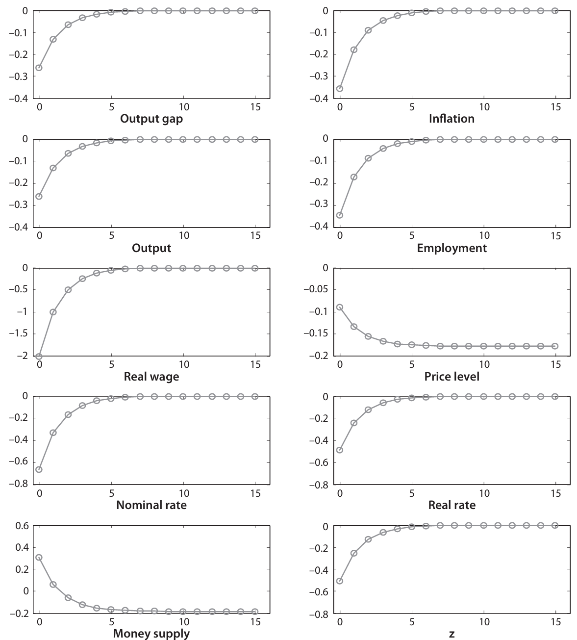
IRF: Monetary policy shock

Impulse response functions to a monetary policy shock from a calibrated version of the model allow to discuss some salient results. An increase of 1% in the interest rate in annualized terms increases the exogenous component by 1%, but output and endogenous variables decrease, so that the final increase in the real interest rate is lower than 1%. In contrast with the classical model, monetary policy shocks and the real interest rate move in the same direction.

The monetary shock utilized for the IRF functions takes the form of an increase of 25 base points in ${ϵ}_t^v$. The increase in the real rate induces effects on consumption through the Euler equation, and thus on aggregate demand and output. This is reflected in the IS equation, where current output gap depends on current and future variables.

The output gap drops, and obviously inflation as well, being related to the output gap. The natural level of output does not change, also reflecting the fact that the output gap is shocked. The real wage also decreases unambiguously, moving down along the labor supply schedule. To solve for the price level, solve $p_t=p_{t-1}+{\pi }_t$ and note that the price level decreases very gradually until stabilization. This is consistent with negative inflation: ultimately, prices stabilize permanently at a lower level (recall, from previous passages, that there is no steady state for prices). To understand this, imagine that a firm sees decreasing demand for their goods: their response will be not only to produce less, but will also lead to lower marginal costs (decreased wage and increased marginal product of labor). Therefore, when they get a chance to adjust prices, they will try to lower prices. Finally, note that money supply also converges to the initial value.

The three predicitons of the classical model conflicting with the empirical evidence are now reversed: non-neutrality of monetary policy, gradual adjustment of the price level, and liquidity effect as all there. The real interest rate is affected by the nominal interest rate because inflation does not move 1-to-1 with due to price stickiness.

IRF: Preference shock

A negative shock to $z_t$ should be interpreted as a negative preference shock: consumers prefer to consume less at the time of the shock. The variables on the column on the left react just the same as in the monetary policy shock, with the exception of the nominal rate and the money supply.

The nominal rate reacts differently through the endogenous component of the policy rule. Inflation and output decrease, and thus the central bank lowers the interest rate. Whenever the nominal rate goes down, so does the real rate, as inflation does not change much. This occurs as an attempt to stabilize the economy, to partly offset the declining demand coming from the preference shock. However, this is not fully offset and the output goes down, although the decrease would have been even larger without the policy intervention.

The money supply goes up in the short run, but not in the long run, because of the lower nominal interest rate. Given this calibration, it tends to offset: $m_t=p_t+{\pi }_t-\eta i_t$, where the first two decrease and the latter increases. For the point of view of the individual firm, this shock looks similar to the monetary policy shock.

IRF: Technology shock

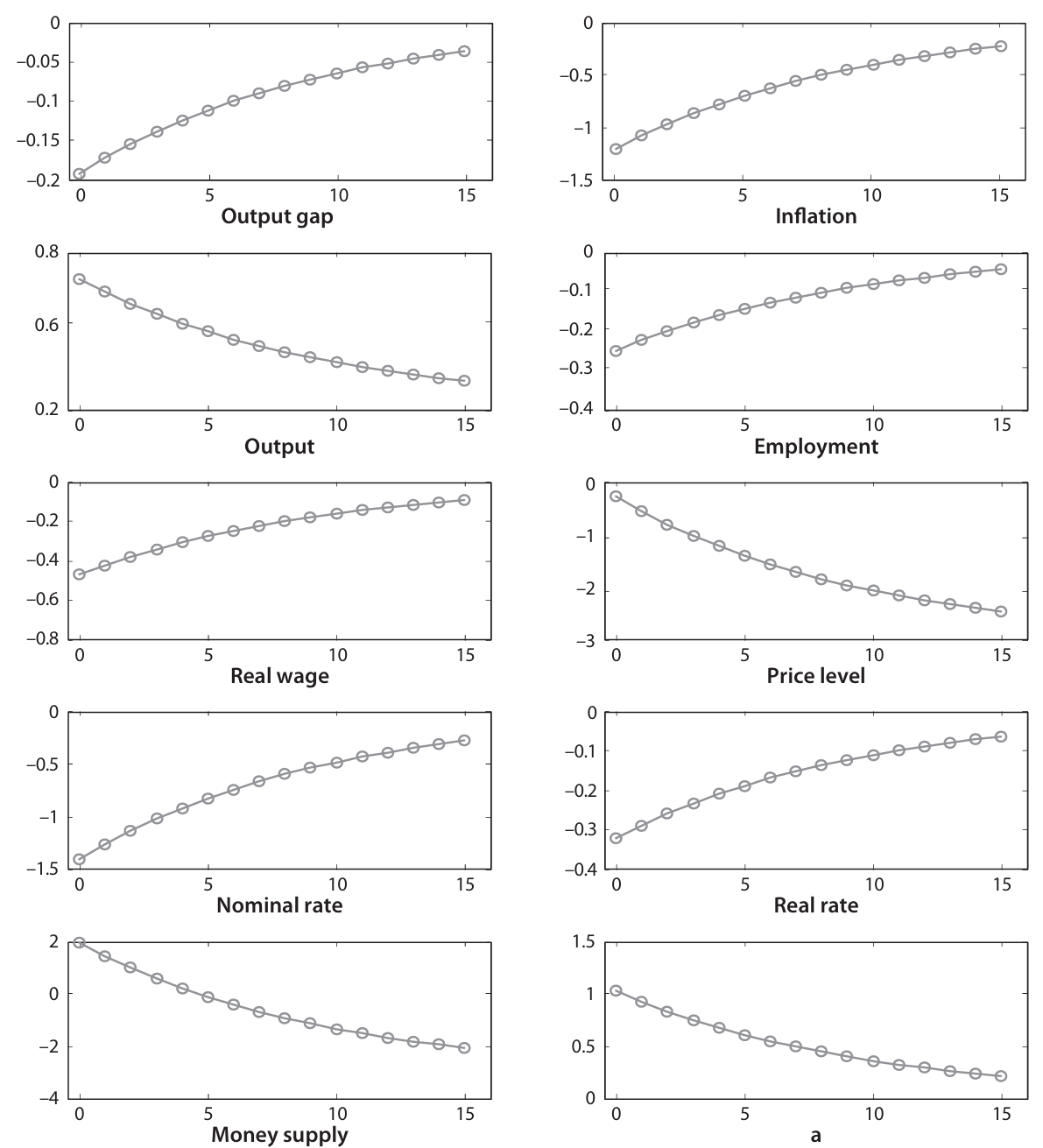
A persistent positive technology shock calls for increased output. However, the output gap decreases and becomes negative. This is due to the fact that output increases by less than the natural level of ouput. Implicitly, this is because the real interest rate does not decrease as much as the natural interest rate — i.e. the central bank is non stimulating the economy enough, under this particular rule and calibration. Inflation, as the output gap, is negative. In principle, the nominal rate responses both to inflation and output, which are now moving in opposite directions. In the present calibration, the nominal rate goes up (the reduction in inflation is dominated by the increase in output). The real wage goes up, but in principle this is ambiguous. In fact, output goes up, but employment decreases in response to a positive technology shock: $w_t=\sigma y_t+\varphi n_t$. Unemployment goes down due to the labor demand equation: $n_t=\frac{y_t-a_t}{1-\alpha }$. If output does not increase as much as technology, as it often happens, then employment decreases. This is a (fairly) general result in NK models: the demand for the good decreases by less than technology, and the firms need less workers than before to produce the, yet higher, quantity demanded by consumers.

Employment and technology shocks in New Keynesian and RBC models

This prediction is at odds with the standard RBC model. A positive technology shock in the RBC would lead to increased employment: if not, those models could not have claimed that they generate business cycles by taking technology shocks as the only source of fluctuation. Thus, the RBC school takes on the tight positive correlation between output and employment. In contrast, the opposite is predicted by the NK model. Empirical evidence does not help much to settle the debate: in the real world, many shocks occur at once, and it is quite difficult to disentangle their relative impact. In Galì (1999), permanent technology shocks found as the only shocks with a permanent effect on labor productivity, which is a feature shared with RBC model. By estimating the impact of these shocks on a number of variables through a SVAR, GDP increases gradually but the total amount of hours worked decrease. This seems to support the NK hypothesis rather than the RBC.

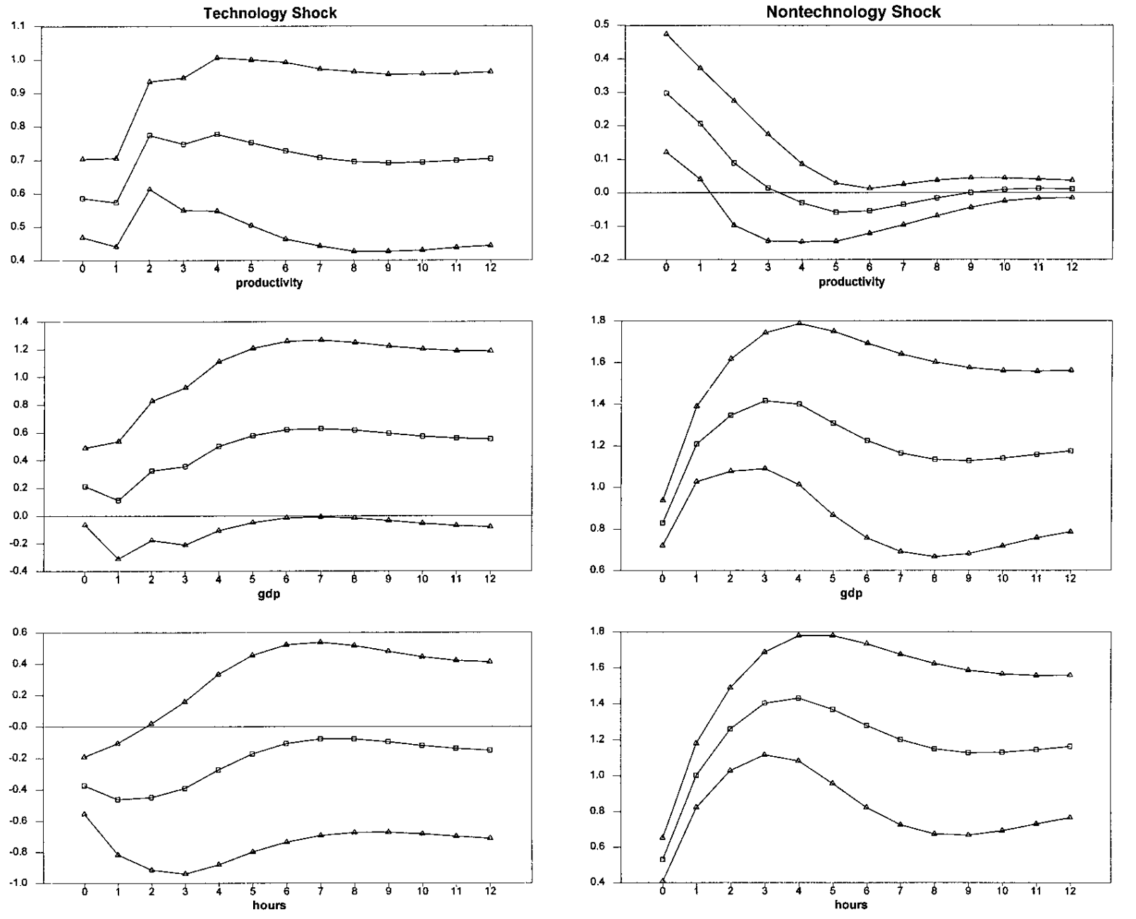
In a related paper, Basu et al. (2006) use actual measures of technology using modified versions of Solow residual’s correcting for problems in increasing returns to scale or non-perfect competition, or observed variations in factors employment. They regress every variable of interest of the current and lagged volumes of the change in technology, and obtain a similar result: a negative correlation between hours worked and technological shocks. This despite using an opposite approach (in Galì, 1999, technology was unobservable and here is a regressor). Note that, under $\sigma =1$, employment will ultimately go back to normal, consistent with balanced growth. Put simply, the following relation must hold in the long run: $c_t+\varphi n_t=\log (1-\alpha )+y_t+n_t$. In this model, $c_t=y_t$, plus the additional feature of the markup: $\varphi n_t=\log (1-\alpha )-n_t-{\mu }_t$; however, the markup also goes back to normal in the long run.

Not only the NK models captures real effects of monetary policy on economic activity: another important message regards the evaluation of models. The main conclusion is that technological shocks should not be a relevant source of fluctuation in the real world. If this were the case, we would observe a negative correlation between output and employment; yet, the opposite is observed. There must be some other, dominant source of fluctuations leading to this stylized fact.

Finally, the NK model highlights that it is not sufficient to compute the second moments of the series and those of the data to validate a model. A more demanding way to test a model is to compare the predictions of a specific shock from the evidence in the data of the same shock, although these are difficult to disentangle in the real world.

Monetary Policy Design

How should monetary policy be designed in a world such as the one described by the New Keynesian model? To answer this question, we introduce a new variable, the welfare-relevant output gap: $x_t\equiv y_t-y_t^e$, where $y_t^e$ is the efficient level of output, i.e. it solves the problem of the social planner (maximizes utility of households) with no prices and no markets and simply resources and technology constraints. By welfare theory, this would correspond to a perfect-competition-no-externality equilibrium. By means of the welfare-relevant output gap, we will consider a second order approximation of the welfare losses. Second-order approximations are usually performed in form of the following second-order Taylor expansion of the log (deviations) of a generic variable from its steady state level, $\frac{X_t-X}{X}\approx {\hat{x}}_t+\frac{1}{2}{\hat{x}}_t^2$. To lighten notation, suppose $U$ denotes steady state utility, $U_t$ denotes time $t$ utility, and $U_t^n$ denotes its natural level at time $t$. Then:

$$\begin{array}{rl}{U}_t-U& \simeq U_c(C_t-C)+U_n(N_t-N)+U_z(Z_t-Z)+\frac{1}{2}{U}_{cc}(C_t-C{)}^2+\frac{1}{2}{U}_{nn}(N_t-N{)}^2+\frac{1}{2}{U}_{zz}(Z_t-Z{)}^2\\ & +U_{cn}(C_t-C)(N_t-N)+U_{cz}(C_t-C)(Z_t-Z)+U_{nz}(N_t-N)(Z_t-Z)+\text{t.i.p.}\\ & \\ & \simeq Z{C}^{-\sigma }(C_t-C)-Z{N}^{\varphi }(N_t-N)+U_z(Z_t-Z)-\frac{1}{2}Z\sigma C^{-\sigma -1}(C_t-C{)}^2-\frac{1}{2}Z\varphi N^{\varphi -1}(N_t-N{)}^2\\ & +\frac{1}{2}{U}_{zz}(Z_t-Z{)}^2+U_{cz}(C_t-C)(Z_t-Z)+U_{nz}(N_t-N)(Z_t-Z)+\text{t.i.p.}\\ & \\ & \simeq Z{C}^{1-\sigma }\left(\frac{C_t-C}{C}\right)-Z{N}^{1+\varphi }\left(\frac{N_t-N}{N}\right)+U_{z}Z\left(\frac{Z_t-Z}{Z}\right)-\frac{1}{2}Z\sigma C^{1-\sigma }{\left(\frac{C_t-C}{C}\right)}^2-\frac{1}{2}Z\varphi N^{1+\varphi }{\left(\frac{N_t-N}{N}\right)}^2\\ & +\frac{1}{2}{U}_{zz}{Z}^2{\left(\frac{Z_t-Z}{Z}\right)}^2+U_{cz}CZ\left(\frac{C_t-C}{C}\right)\left(\frac{Z_t-Z}{Z}\right)+U_{nz}NZ\left(\frac{N_t-N}{N}\right)\left(\frac{Z_t-Z}{Z}\right)+\text{t.i.p.}\\ & \\ & \simeq Z{C}^{1-\sigma }({\hat{c}}_t+\frac{1}{2}{\hat{c}}_t^2)-Z{N}^{1+\varphi }({\hat{n}}_t+\frac{1}{2}{\hat{n}}_t^2)+U_{z}Z{z}_t+\frac{1}{2}{U}_{zz}{Z}^2{z}_t^2-\frac{1}{2}Z\sigma C^{1-\sigma }{\hat{c}}_t^2-\frac{1}{2}Z\varphi N^{1+\varphi }{\hat{n}}_t^2\\ & +U_{cz}CZ{\hat{c}}_t{z}_t+U_{nz}NZ{\hat{n}}_t{z}_t+\text{t.i.p.}\\ & \\ & \simeq Z{C}^{1-\sigma }{\hat{c}}_t-Z{N}^{1+\varphi }{\hat{n}}_t+U_{z}Z{z}_t+\frac{1}{2}Z{C}^{1-\sigma }(1-\sigma ){\hat{c}}_t^2-\frac{1}{2}Z{N}^{1+\varphi }(1+\varphi ){\hat{n}}_t^2+\frac{1}{2}{U}_{zz}{Z}^2{z}_t^2\\ & +U_{cz}CZ{\hat{c}}_t{z}_t+U_{nz}NZ{\hat{n}}_t{z}_t+\text{t.i.p.}\\ & \\ & \simeq Z{C}^{1-\sigma }\left({\hat{c}}_t(1+z_t)+\frac{1-\sigma }{2}{\hat{c}}_t^2\right)-Z{N}^{1+\varphi }({\hat{n}}_t(1+z_t)+\frac{1+\varphi }{2}{\hat{n}}_t^2)+\text{t.i.p.}\\ U_t-U& \simeq U_{c}C\left({\hat{y}}_t(1+z_t)+\frac{1-\sigma }{2}{\hat{y}}_t^2\right)+U_{n}N\left({\hat{n}}_t(1+z_t)+\frac{1+\phi }{2}{\hat{n}}_t^2\right)\end{array}$$

where the term $\text{t.i.p.}$ stands for terms independent of policy. Observe that, since $N_t={\left(\frac{Y_t}{A_t}\right)}^{\frac{1}{1-\alpha }}{\int }_0^1{\left(\frac{P_t(i)}{P_t}\right)}^{-\frac{ϵ}{1-\alpha }}di$, then $(1-\alpha ){\hat{n}}_t={\hat{y}}_t-a_t+d_t$. In the neighborhood of a symmetric steady state and up to a second order approximation, $d_t=\frac{ϵ}{2\Theta }{\text{var}}_i(p_t(i))$ — a result previously proved in the derivation of cross-sectional price dispersion. Thus:

$$\begin{array}{rl}{U}_t-U& \simeq U_{c}C\left({\hat{y}}_t(1+z_t)+\frac{1-\sigma }{2}{\hat{y}}_t^2\right)+\frac{U_{n}N}{1-\alpha }\left({\hat{y}}_t(1+z_t)+\frac{ϵ}{2\Theta }{\text{var}}_i(p_t(i))+\frac{1+\phi }{2(1-\alpha )}({\hat{y}}_t-a_t{)}^2\right)+\text{t.i.p.}\end{array}$$

Last, observing that efficiency of the steady state implies that $-\frac{U_n}{U_c}=\text{MPN}=(1-\alpha )\frac{Y=C}{N}$:

$$\begin{array}{rl}\frac{U_t-U}{U_{c}C}& \simeq {\hat{y}}_t(1+z_t)+\frac{1-\sigma }{2}{\hat{y}}_t^2+\underset{=-1}{\underbrace{\frac{U_{n}N}{(1-\alpha )U_{c}C}}}\left({\hat{y}}_t(1+z_t)+\frac{ϵ}{2\Theta }{\text{var}}_i(p_t(i))+\frac{1+\phi }{2(1-\alpha )}({\hat{y}}_t-a_t{)}^2\right)+\text{t.i.p.}\\ & \simeq {\hat{y}}_t(1+z_t)+\frac{1-\sigma }{2}{\hat{y}}_t^2-{\hat{y}}_t(1+z_t)-\frac{ϵ}{2\Theta }{\text{var}}_i(p_t(i))-\frac{1+\phi }{2(1-\alpha )}({\hat{y}}_t-a_t{)}^2+\text{t.i.p.}\\ & \simeq \frac{1-\sigma }{2}{\hat{y}}_t^2-\frac{ϵ}{2\Theta }{\text{var}}_i(p_t(i))-\frac{1+\phi }{2(1-\alpha )}({\hat{y}}_t-a_t{)}^2+\text{t.i.p.}\\ & \simeq -\frac{1}{2}\left[\frac{ϵ}{\Theta }{\text{var}}_i(p_t(i))-(1-\sigma ){\hat{y}}_t^2+\frac{1+\phi }{(1-\alpha )}({\hat{y}}_t-a_t{)}^2\right]+\text{t.i.p.}\\ & \simeq \frac{1-\sigma }{2}{\hat{y}}_t^2-\frac{ϵ}{2\Theta }{\text{var}}_i(p_t(i))-\frac{1+\phi }{2(1-\alpha )}({\hat{y}}_t-a_t{)}^2+\text{t.i.p.}\\ & \simeq -\frac{1}{2}\left[\frac{ϵ}{\Theta }{\text{var}}_i(p_t(i))+\left(\sigma +\frac{\varphi +\alpha }{1-\alpha }\right){\hat{y}}_t^2-2\left(\frac{1+\phi }{(1-\alpha )}\right){\hat{y}}_t{a}_t\right]+\text{t.i.p.}\\ & \simeq -\frac{1}{2}\left[\frac{ϵ}{\Theta }{\text{var}}_i(p_t(i))+\left(\sigma +\frac{\varphi +\alpha }{1-\alpha }\right)({\hat{y}}_t^2-2{\hat{y}}_t{\hat{y}}_t^n)\right]+\text{t.i.p.}\\ & \simeq -\frac{1}{2}\left[\frac{ϵ}{\Theta }{\text{var}}_i(p_t(i))+\left(\sigma +\frac{\varphi +\alpha }{1-\alpha }\right){\tilde{y}}_t^2\right]+\text{t.i.p.}\end{array}$$

exploiting the fact that ${\hat{y}}_t^n=\frac{1+\varphi }{\sigma (1-\alpha )+\varphi +\alpha }{a}_t-\stackrel{\text{t.i.p.}}{\overbrace{\frac{(1-\alpha )[\log (1-\alpha )+\mu ]}{1+\varphi }}}$ (the details of this equation can be found in the derivation of employment, real wages, and the real rate). Finally, the welfare loss resulting from fluctuations from the steady state can be written as:

$$\begin{array}{rl}\mathbb{W}& \equiv -{\mathbb{E}}_0\sum _{t=0}^{\infty }{\beta }^t\frac{U_t-U}{U_{c}C}\\ & \approx \frac{1}{2}{\mathbb{E}}_0\sum _{t=0}^{\infty }{\beta }^t\left[\frac{ϵ}{\Theta }{\text{var}}_i(p_t(i))+\left(\sigma +\frac{\varphi +\alpha }{1-\alpha }\right){\tilde{y}}_t^2\right]\\ & \approx \frac{1}{2}{\mathbb{E}}_0\sum _{t=0}^{\infty }{\beta }^t\left[\frac{ϵ}{\lambda }{\pi }_t^2+\left(\sigma +\frac{\varphi +\alpha }{1-\alpha }\right){\tilde{y}}_t^2\right]\end{array}$$

An implication of this equation is that an optimal policy — a policy that minimizes the welfare loss — must enforce zero inflation (as we anticipated in deriving the NKPC in the previous chapter) and zero output gap. If the SS were efficient, in equilibrium the following identity would hold: $\text{MRS}=\text{MPN}$. In case of inefficiency, however, they will differ: for reasons that will be clarified in the future, MPN is usually larger than MRS. Therefore, the output gap will very hardly be zero. In turn, the average welfare loss will depend on a linear combination of the variances of the output gap and inflation:

$$\mathbb{L}=\frac{1}{2}\left[\left(\sigma +\frac{\varphi +\alpha }{1-\alpha }\right)\text{var}({\tilde{y}}_t)+\frac{ϵ}{\lambda }\text{var}({\pi }_t)\right]$$

Note that the relative weight of output gap fluctuations in the loss function is increasing in $\sigma$, $\varphi$, and $\alpha$. The reason is that larger values of those “curvature” parameters amplify the effect of any given deviation of output from its natural (efficient) level on the size of the gap between the marginal rate of substitution and the marginal product of labor, which is a measure of the economy’s aggregate inefficiency. On the other hand, the weight of inflation fluctuations is increasing in the elasticity of substitution among goods, since the latter amplifies the dispersion in the quantities of goods consumed of different varieties caused by any given price dispersion. The inflation weight is also increasing in the degree of price stickiness $\theta$ (which is inversely related to $\lambda$), since a greater stickiness amplifies the degree of price dispersion associated with any given deviation from zero inflation.

Let us consider the solution to this problem in two environments: in the efficient natural equilibrium, a case unrealistic in practice but with a simple benchmark solution where the only source of inefficiency is the presence of sticky prices, and in an inefficient natural equilibrium, where the other imperfections add to the economy on top of sticky prices.

Efficient Natural Equilibrium

In case of an efficient equilibrium, the only distortion in the economy lies in sticky prices. An equilibrium is efficient if at all times, not only in the steady state, the efficient output is equal to the natural level of output. This grounds the first theoretical justification for price stability: price stability makes it optimal for efficient equilibria to be implemented and minimize welfare. How can the central bank bring about this optimal outcome as an equilibrium? That is, ensure that inflation in 0? The optimal rule:

$$i_t=r_t^n+{\varphi }_{\pi }{\pi }_t$$

must be such that, when plugged into the Dynamic IS equation and the NKPC, it yields: ${\tilde{y}}_t={\mathbb{E}}_t[{\tilde{y}}_{t+1}]-\frac{1}{\sigma }[{\varphi }_{\pi }{\pi }_t-{\mathbb{E}}_t[{\pi }_{t+1}]]$ Which is solved at 0 inflation. Is it, however, the unique solution? For a coefficient ${\varphi }_{\pi }>1$, the solution is unique, as discussed in Chapter 1. The practical problem with this rule, however, is that a central bank may not be able to follow it, since the natural interest rate is not observed and is rather a theoretical concept. In actual practice, interest rate rules must be “simple”, and definitely not rely on an unobservable and hardly imputable state of the economy.

Are there any simple rules approximating the optimal rule? This question fueled a large body of recent research in monetary macroeconomics. The criterion to evaluate simple rules is exactly the welfare loss previously derived and originally proposed by Woodford (2003). Let us consider the Taylor rule based on this benchmark.

Taylor rule

$i_t=\rho +{\varphi }_{\pi }{\pi }_t+{\varphi }_y{\hat{y}}_t$

Simulating the model under such rule and proper calibrations of the parameters, the welfare loss can be computed based on the output gap and inflation. Consider both the technology shock and demand shock, and see how the rule behaves conditional on each shock separately. We’ll consider the benchmark values proposed by Taylor, namely ${\varphi }_{\pi }=1.5$ and ${\varphi }_y=0.125$. The table computes the welfare loss, which can be interpreted as the loss that a consumer is willing to internalize in order to get rid of fluctuations.

	Technology				Demand
${\varphi }_{\pi }$	1.5	1.5	5	1.5	1.5	1.5	5	1.5
${\varphi }_y$	0.125	0	0	1	0.125	0	0	1
$\sigma (y)$	1.85	2.07	2.25	1.06	0.59	0.68	0.28	0.31
$\sigma (\tilde{y})$	0.44	0.21	0.03	1.23	0.59	0.68	0.28	0.31
$\sigma (\pi )$	0.69	0.34	0.05	1.94	0.20	0.23	0.09	0.10
$\mathbb{L}$	1.02	0.25	0.006	7.98	0.10	0.13	0.02	0.02

Consider a rule with parameters 1.5/0. Of course, the volatility of output increases; however, the volatility of output gap and inflation decrease. Through the lens of the model, this is an improvement: welfare losses depend on output gap and inflation, not output. Move on to calibration 5/0, that is: A very aggressive central bank increases the volatility of output even more, but output gap, inflation, and welfare losses are basically 0. Last, if the central bank stabilizes outcome aggressively (1.5/1), the welfare loss becomes very large. We may erroneously conclude that responding to output is not desirable, while responding to inflation is. However, this depends on the fact that there fluctuations are technological, and technology only affects the natural level of output. A stabilizing output means that the output gap is de-stabilized, as the gap cannot simply follow the movement of output itself. Ideally, we’d like to steer output so that it follows its natural level, rather than diverging from it. Let us now turn to demand shocks. In this scenario, ignoring output is not optimal, as it leads to fluctuations in the output gap and inflation. By increasing the output coefficient over Taylor’s benchmark, a very efficient rule is obtained. This is because we introduced preference shocks, a type of shock that does not affect output. By stabilizing output, the central bank is actually stabilizing the output gap and inflation, altogether and all at once.

In the real world, however, the two types of shocks occur at the same time, and the central bank may not be able to perfectly decompose them. In light of the previous reasoning, a central bank should focus on inflation: this is the dimension that does well with both shocks, while stabilizing output can be detrimental if the shocks are due to technological shifts and wrongly interpreted as demand shocks. Moreover, the output gap is not directly observed. Ultimately, then, these two arguments justify the central banks’ focus on inflation targeting. In fact, in the limit, a policy with ${\varphi }_y=0$ and ${\varphi }_{\pi }\to \infty$ would be such that both 0 inflation and 0 output gap would hold. In practice, this is not credible as minimal fluctuations due to measurement errors would imply an enormous responses by the central bank.

Why is inflation bad in this economy? In fact, it does not appear in households utility. The fundamental reason is that inflation generates price dispersion. In an inflationary environment, some firms are adjusting prices; but by assumption only a fraction of firm can be doing that, leading to dispersion. If the deviation from 0 is very large, then these firms are adjusting by a lot. However, price dispersion necessarily generates quantity dispersion among various types of goods, where these would, in turn, enter the utility function symmetrically and using an identical technology. Price fluctuations lead to fluctuations in the composition of consumption. While the social planner would choose equal proportion of these goods, firms produce different quantities, hire different quantities of labor. Then, firms with low prices will (temporarily) also occupy more labor. In fact, in the function $\mathbb{L}$ $ϵ$ is present, telling the extent to which price dispersion is reflected in quantity dispersion. In contrast, it is inversely correlated with $\lambda$: if price stickiness is strong and $\theta$ is large, in order to achieve a given level of inflation, a larger dispersion of prices will follow, as a smaller fraction of firm adjust prices at any period. In monetary economics, there is a long standing belief that inflation induces other types of losses, typically of transactionary kind. With its minimal assumptions on utility and monopolistic competition, however, this is the kind of losses that the New Keynesian model predicts.

Inefficient Natural Equilibrium

In the case of an infficient natural equilibrium, even if prices were flexible, the outcome would not be optimal, meaning that some additional distortions must be present on top of sticky prices (labor markets, taxation, externalities…). If so, the standard output gap and the welfare relevant output gap no longer coincide: $y_t^n\ne y_t^e$. Recall that the welfare output gap is the relevant level of output for optimal monetary policy — the NKPC is, in fact, expressed in terms of the standard output gap. To begin with, rewrite the NKPC in terms of the welfare relevant output gap,by first noting that ${\tilde{y}}_t={\hat{y}}_t-{\hat{y}}_t^n=({\hat{y}}_t-{\hat{y}}_t^e)+({\hat{y}}_t^e-{\hat{y}}_t^n)=x_t+\frac{u_t}{\kappa }$ by adding and subtracting the deviations of the efficient level of output from its steady state:

$$\begin{array}{c}{\pi }_t=\beta {\mathbb{E}}_t[{\pi }_{t+1}]+\kappa {\hat{x}}_t+u_t\end{array}$$

The output gap was replaced by the welfare-relevant output gap $\hat{x}\equiv {\hat{y}}_t-{\hat{y}}_t^e$ and the cost push shock $u_t\equiv \kappa ({\hat{y}}_t^e-{\hat{y}}_t^n)$ which is independent of monetary policy since the natural level of output is not affected by shocks nor by fluctuations in the efficient output gap (which solves the social planner’s problem). Fluctuations in $u_t$ can be interpreted as shocks in presence of distortions or imperfections that make the economy respond inefficiently to the shock despite price flexibility. The cost push shocks will fluctuate because the natural level of output may respond differently than the efficient level of output due to some distortionary inefficiency.

Types of Output

• Output ($y_t$): The actual level of output in the economy at time $t$. In log-linearized form, ${\hat{y}}_t$ is the percent deviation of output from its steady state.
• Natural Level of Output ($y_t^n$): The level of output with flexible prices but other distortions (e.g., monopolistic competition). Its log-linearized form is ${\hat{y}}_t^n$.
• Efficient Level of Output ($y_t^e$): The socially optimal level of output that a benevolent social planner would choose (i.e., with flexible prices and no other distortions). Its log-linearized form is ${\hat{y}}_t^e$.
• Standard Output Gap (${\tilde{y}}_t$): The gap between actual and natural output. This is the gap that appears in the standard NKPC.
  • ${\tilde{y}}_t={\hat{y}}_t-{\hat{y}}_t^n$
• Welfare-Relevant Output Gap ($x_t$): The gap between actual and efficient output. This is the gap that matters for welfare analysis.
  • $x_t={\hat{y}}_t-{\hat{y}}_t^e$
• Cost-Push Shock ($u_t$): A shock term that arises when the NKPC is expressed in terms of the welfare-relevant output gap. It captures the distortions that cause the natural and efficient levels of output to diverge.
  • $u_t=\kappa ({\hat{y}}_t^e-{\hat{y}}_t^n)$

The welfare loss under an inefficient economy is derived as follows. Starting from ^e998e0:

$$U_t-U\simeq U_{c}C\left({\hat{y}}_t(1+z_t)+\frac{1-\sigma }{2}{\hat{y}}_t^2\right)+\frac{U_{n}N}{1-\alpha }\left({\hat{y}}_t(1+z_t)+\frac{ϵ}{2\Theta }{\text{var}}_i(p_t(i))+\frac{1+\phi }{2(1-\alpha )}({\hat{y}}_t-a_t{)}^2\right)+\text{t.i.p.}$$

Let $\Phi$ denote the size of the steady state distortion. This is defined implicitly by $-\frac{U_n}{U_c}=\text{MPN}(1-\Phi )$. Under the “small distortion” assumption, so that the product $\Phi$ with a second-order term can be taken as neglibigle:

$$\begin{array}{rl}\frac{U_t-U}{U_{c}C}& ={\hat{y}}_t(1+z_t)+\frac{1-\sigma }{2}{\hat{y}}_t^2-(1-\Phi )\left({\hat{y}}_t(1+z_t)+\frac{ϵ}{2\Theta }{\text{var}}_i(p_t(i))+\frac{1+\phi }{2(1-\alpha )}({\hat{y}}_t-a_t{)}^2\right)+\text{t.i.p.}\\ & =\left({\hat{y}}_t+{\hat{y}}_t{z}_t\right)+\frac{1-\sigma }{2}{\hat{y}}_t^2-(1-\Phi )\left({\hat{y}}_t+{\hat{y}}_t{z}_t\right)-(1-\Phi )\left(\frac{ϵ}{2\Theta }{\text{var}}_i(p_t(i))+\frac{1+\phi }{2(1-\alpha )}({\hat{y}}_t-a_t{)}^2\right)+\text{t.i.p.}\\ & =({\hat{y}}_t-(1-\Phi ){\hat{y}}_t)+({\hat{y}}_t{z}_t-(1-\Phi ){\hat{y}}_t{z}_t)+\frac{1-\sigma }{2}{\hat{y}}_t^2-(1-\Phi )\left(\frac{ϵ}{2\Theta }{\text{var}}_i(p_t(i))+\frac{1+\phi }{2(1-\alpha )}({\hat{y}}_t-a_t{)}^2\right)+\text{t.i.p.}\\ & =\Phi {\hat{y}}_t+\Phi ({\hat{y}}_t{z}_t)+\frac{1-\sigma }{2}{\hat{y}}_t^2-(1-\Phi )\left(\frac{ϵ}{2\Theta }{\text{var}}_i(p_t(i))+\frac{1+\phi }{2(1-\alpha )}({\hat{y}}_t-a_t{)}^2\right)+\text{t.i.p.}\end{array}$$

Neglecting terms that are products of small deviations or independent of policy (like $z_t$ and the cross-term $\Phi {\hat{y}}_t{z}_t$):

$$\begin{array}{rl}& \simeq \Phi {\hat{y}}_t+\frac{1-\sigma }{2}{\hat{y}}_t^2-\frac{1+\phi }{2(1-\alpha )}({\hat{y}}_t-a_t{)}^2-\frac{ϵ}{2\Theta }{\text{var}}_i(p_t(i))+\text{t.i.p.}\\ & \simeq \Phi {\hat{y}}_t-\frac{1}{2}\left[\left(\sigma +\frac{\phi +\alpha }{1-\alpha }\right)({\hat{y}}_t-{\hat{y}}_t^n{)}^2+\frac{ϵ}{\Theta }{\text{var}}_i(p_t(i))\right]+\text{t.i.p.}\\ & \simeq \Phi {\tilde{y}}_t-\frac{1}{2}\left[\left(\sigma +\frac{\phi +\alpha }{1-\alpha }\right){\tilde{y}}_t^2+\frac{ϵ}{\Theta }{\text{var}}_i(p_t(i))\right]+\text{t.i.p.}\end{array}$$

Let ${\tilde{y}}_t\equiv {\hat{x}}_t\text{ and use }{\text{var}}_i(p_t(i))=\frac{\Theta }{\lambda }{\pi }_t^2$. The welfare loss is $\mathbb{W}=-{\mathbb{E}}_0{\sum }_{t=0}^{\infty }{\beta }^t\left(\frac{U_t-U}{U_{c}C}\right)$, that is:

$$\begin{array}{rl}\mathbb{W}& \simeq -{\mathbb{E}}_0\sum _{t=0}^{\infty }{\beta }^t\left[\Phi {\hat{x}}_t-\frac{1}{2}\left(\left(\sigma +\frac{\phi +\alpha }{1-\alpha }\right){\hat{x}}_t^2+\frac{ϵ}{\lambda }{\pi }_t^2\right)\right]+\text{t.i.p}\\ & \simeq {\mathbb{E}}_0\sum _{t=0}^{\infty }{\beta }^t\left[-\Phi {\hat{x}}_t+\frac{1}{2}\left(\sigma +\frac{\phi +\alpha }{1-\alpha }\right){\hat{x}}_t^2+\frac{ϵ}{2\lambda }{\pi }_t^2\right]+\text{t.i.p}\\ & \simeq \frac{1}{2}{\mathbb{E}}_0\sum _{t=0}^{\infty }{\beta }^t\left[\frac{ϵ}{\lambda }{\pi }_t^2+\left(\sigma +\frac{\phi +\alpha }{1-\alpha }\right){\hat{x}}_t^2-2\Phi {\hat{x}}_t\right]+\text{t.i.p}\end{array}$$

following the same derivation as ^0c3714, ^4c6b9a and ^d46b92 , using the additional fact that ${\hat{y}}_t^e\equiv y_t^e-y^e$ and thus ${\hat{y}}_t^e=\frac{1+\varphi }{\sigma (1-\alpha )+\varphi +\alpha }{a}_t$ (also, dropping the $1+z_t$ term as independent of monetary policy³). By assuming an efficient steady state, i.e., $\Phi =0$, this case in entirely analogous to the efficient natural equilibrium. Note that this problem is entirely proportional to the following:

$$\min {\mathbb{E}}_0\sum _{t=0}^{\infty }{\beta }^t({\pi }_t^2+\vartheta x_t^2)\text{ such that }{\pi }_t=\beta {\mathbb{E}}_t[{\pi }_{t+1}]+\kappa x_t+u_t$$

for an exogenous $u_t={\rho }_u{u}_{t-1}+{ϵ}_t$ with $\vartheta$ representing the weight of output gap fluctuations relative to inflation in the loss function and welfare-theoretically equal to the utilithy based $\vartheta =\left(\sigma +\frac{\varphi +\alpha }{1-\alpha }\right)\frac{\lambda }{ϵ}=\frac{\kappa }{ϵ}$. Alternatively, interpret $\vartheta$ arbitrary central bank preference towards output gap rather tha prices. Additional assumptions should be make on how the central bank can affect the expectations. Two assumption will be proposed. In one case, the central bank cannot influence the expectations of future variables.

Optimal Monetary Policy under Discretion

If the central bank cannot influence the expectations of future variables, then the problem can be transformed into a static problem where the central bank takes expected inflation as given and responds optimally through the NKPC. The solution is obtained at:

$$\begin{array}{rlr}& \underset{x_t,{\pi }_t}{\min }{\pi }_t^2+\vartheta x_t^2& \text{ such that }{\pi }_t=\kappa x_t+v_t\\ =& \underset{x_t}{\min }(\kappa x_t+v_t{)}^2+\vartheta x_t^2& \end{array}$$

with optimality condition given by $x_t=-\frac{\kappa }{\vartheta }{\pi }_t$. This is known as the targeting rule, which focuses not on the instruments of monetary policy but rather on the target variables. This rule should offset inflation by generating a recession (lowering the output gap), so that it also lowers inflation. The larger is $\vartheta$, the smaller the recession. To find the corresponding equilibrium, take the NKPC and plug in the optimal $x_t$; after obtaining the corresponding difference equation in ${\pi }_t$, solve by iterating forward:

$$\begin{array}{rl}{\pi }_t& =\beta {\mathbb{E}}_t[{\pi }_{t+1}]+\kappa x_t+u_t\\ & =\beta {\mathbb{E}}_t[{\pi }_{t+1}]-\frac{{\kappa }^2}{\vartheta }{\pi }_t+u_t\\ & =\frac{\beta \vartheta }{{\kappa }^2+\vartheta }{\mathbb{E}}_t[{\pi }_{t+1}]+\frac{\vartheta }{{\kappa }^2+\vartheta }{u}_t\\ & \\ & \{\begin{array}{ll}{\mathbb{E}}_t[u_{t+1}]& ={\rho }_u{u}_t\\ {\mathbb{E}}_t[{\pi }_{t+1}]& =\frac{\beta \vartheta }{{\kappa }^2+\vartheta }{\mathbb{E}}_t[{\pi }_{t+2}]+\frac{\vartheta {\rho }_u}{{\kappa }^2+\vartheta }{u}_t\end{array}\\ & \\ {\pi }_t& =\frac{\beta \vartheta }{{\kappa }^2+\vartheta }\left(\frac{\beta \vartheta }{{\kappa }^2+\vartheta }{\mathbb{E}}_t[{\pi }_{t+2}]+\frac{\vartheta {\rho }_u}{{\kappa }^2+\vartheta }{u}_t\right)+\frac{\vartheta }{{\kappa }^2+\vartheta }{u}_t\\ {\pi }_t& ={\left(\frac{\beta \vartheta }{{\kappa }^2+\vartheta }\right)}^2{\mathbb{E}}_t[{\pi }_{t+2}]+\frac{\vartheta (\beta \vartheta {\rho }_u+{\kappa }^2+\vartheta )}{({\kappa }^2+\vartheta {)}^2}{u}_t\\ {\pi }_t& ={\left(\frac{\beta \vartheta }{{\kappa }^2+\vartheta }\right)}^j{\mathbb{E}}_t[{\pi }_{t+j}]+\sum _{i=0}^{j-1}{\left(\frac{\beta \vartheta }{{\kappa }^2+\vartheta }\right)}^i\frac{\vartheta }{{\kappa }^2+\vartheta }{\mathbb{E}}_t[u_{t+i}]\\ {\pi }_t& =\frac{\vartheta }{{\kappa }^2+\vartheta }\sum _{i=0}^{\infty }{\left(\frac{\beta \vartheta {\rho }_u}{{\kappa }^2+\vartheta }\right)}^i{u}_t\\ {\pi }_t& =\frac{\vartheta }{{\kappa }^2+\vartheta }\frac{1}{1-\frac{\beta \vartheta {\rho }_u}{{\kappa }^2+\vartheta }}{u}_t\\ {\pi }_t& =\frac{\vartheta }{{\kappa }^2+\vartheta -\beta \vartheta {\rho }_u}{u}_t\\ {\pi }_t& =\frac{\vartheta }{{\kappa }^2+\vartheta (1-\beta {\rho }_u)}{u}_t\end{array}$$

which can be summarized in the following equilibrium:

$$\{\begin{array}{l}{\pi }_t=\frac{\vartheta }{{\kappa }^2+\vartheta (1-\beta {\rho }_u)}{u}_t\\ x_t=\frac{\kappa }{{\kappa }^2+\vartheta (1-\beta {\rho }_u)}{u}_t\\ i_t=r_t^e+\frac{\vartheta {\rho }_u+\sigma \kappa (1-{\rho }_u)}{{\kappa }^2+\vartheta (1-\beta {\rho }_u)}{u}_t\end{array}$$

This is sometimes referred to as time-consistent policy: there is no sense in which the central bank may be tempted to break past promises — indeed, it doesn’t make any exception. In presence of a cost push shock, a central bank following this rule should respond by letting inflation increase, but not completely: in fact, it is calling at the same time for a negative output gap, engineering a recession, which tends to dampen the inflationary pressures. Another way to put this is that the central bank redistributes the costs between the output gap and inflation, since the losses are convex in either variable.

Note that, however, the interest rate rule in ^4a5398 does not guarantee a unique equilibrium, as the price dynamics might be indetermined. To uniquely pin down an equilibrium, implement the rule by rewriting the expression and appending a term proportional to the deviation of inflation from its desired level:

$$\begin{array}{rl}{i}_t& =r_t^e+\frac{\vartheta {\rho }_u+\sigma \kappa (1-{\rho }_u)}{{\kappa }^2+\vartheta (1-\beta {\rho }_u)}{u}_t+{\varphi }_{\pi }\left({\pi }_t-\frac{\vartheta }{{\kappa }^2+\vartheta (1-\beta {\rho }_u)}{u}_t\right)\\ & =r_t^e+\Theta u_t+{\varphi }_{\pi }{\pi }_t\end{array}$$

for $\Theta =\frac{\sigma \kappa (1-{\rho }_u)-\vartheta ({\varphi }_{\pi }-{\rho }_u)}{{\kappa }^2+\vartheta (1-\beta )}$. Ex post, in equilibrium, the term in brackets will be 0, but it is the one that guarantess uniqueness: the central bank has to threaten to increase $i$ sufficiently if inflation deviates from the desired path.

Optimal Monetary Policy under Commitment

In this other case, the central bank commits itself to a plan in period 0 which is state-contingent but provides a specification for all subsequent periods in all scenarios and moves of nature. Afterwards, it just implements the plan. The central bank may be tempted to deviate, but we assume the central bank sticks to the plan by assumption of commitment. In so doing, the central bank can affect expectations of future variables. The central bank solve the state-contingent plan that minimizes the loss function subject to the sequence of constraints:

$$\begin{array}{r}\underset{\{x_t,{\pi }_t{\}}_{t=0}^{\infty }}{\min }{\beta }^t({\pi }_t^2+\vartheta x_t^2)\text{ such that }{\pi }_t=\beta {\mathbb{E}}_t[{\pi }_{t+1}]+\kappa x_t+u_t\end{array}$$

Set up the Lagrangian (for each period) and solve for the optimality conditions:

$$\mathcal{L}={\mathbb{E}}_0\sum _{t=0}^{\infty }{\beta }^t\left[\frac{1}{2}(p_t^2+\vartheta x_t^2)+{\xi }_t({\pi }_t-\kappa x_t-\beta {\pi }_{t+1})\right]$$

Note that the exogenous error term disappears by the law of iterated expectations (i.e., ${\mathbb{E}}_0[{\mathbb{E}}_t[{\pi }_{t+1}]]={\mathbb{E}}_0[{\pi }_{t+1}]$). The optimality conditions are as follows:

$$\{\begin{array}{l}\vartheta x_t-\kappa {\xi }_t=0\\ {\pi }_t+{\xi }_t-{\xi }_{t-1}=0\end{array}$$

assuming ${\xi }_{0-1}=0$, which implies ${\xi }_0=-{\pi }_0$. Combining the two constraints to eliminate the Lagrangian multipliers, note that at time 0:

$$\begin{array}{rl}{x}_0& =-\frac{\kappa }{\vartheta }{\pi }_0\\ x_1-x_0& =x_0-\frac{\kappa }{\vartheta }{\pi }_1-x_0\\ \Delta x_1& =-\frac{\kappa }{\vartheta }{\pi }_1\end{array}$$

Generalizing for any $t$:

$$\begin{array}{rl}{x}_t& =x_0-\frac{\kappa }{\vartheta }\sum _{j=0}^t{\pi }_j\\ x_t& =-\frac{\kappa }{\vartheta }(p_t-p_{-1})\\ x_t& =-\frac{\kappa }{\vartheta }{\hat{p}}_t\end{array}$$

Combining this result with ^aa7e11:

$$\begin{array}{rl}{\pi }_t& =\beta {\mathbb{E}}_t[{\pi }_{t+1}]+\kappa {\hat{x}}_t+u_t\\ & =\beta {\mathbb{E}}_t[{\pi }_{t+1}]+\kappa ({\hat{y}}_t-{\hat{y}}_t^n)+u_t\end{array}$$

and taking ^26558a plugged into the Dynamic IS ^1d20a7:

$$\begin{array}{rl}\Delta p_t& \equiv p_t-p_{-1}\\ {\pi }_t& =(p_t-p_{-1})-(p_{t-1}-p_{-1})=\Delta p_t-\Delta p_{t-1}\\ {\pi }_{t+1}& =\Delta p_{t+1}-\Delta p_t\\ \Delta p_t-\Delta p_{t-1}& =\beta {\mathbb{E}}_t[\Delta p_{t+1}-\Delta p_t]+\kappa x_t+u_t\\ \Delta p_t-\Delta p_{t-1}& =\beta {\mathbb{E}}_t[\Delta p_{t+1}]-\beta \Delta p_t-\frac{{\kappa }^2}{\vartheta }\Delta p_t+u_t\\ \Delta p_t+\beta \Delta p_t+\frac{{\kappa }^2}{\vartheta }\Delta p_t& =\Delta p_{t-1}+\beta {\mathbb{E}}_t[\Delta p_{t+1}]+u_t\\ \Delta p_t\left(1+\beta +\frac{{\kappa }^2}{\vartheta }\right)& =\Delta p_{t-1}+\beta {\mathbb{E}}_t[\Delta p_{t+1}]+u_t\\ \Delta p_t\left(\frac{\vartheta (1+\beta )+{\kappa }^2}{\vartheta }\right)& =\Delta p_{t-1}+\beta {\mathbb{E}}_t[\Delta p_{t+1}]+u_t\\ \Delta p_t& =\frac{\vartheta }{\vartheta (1+\beta )+{\kappa }^2}\Delta p_{t-1}+\frac{\vartheta \beta }{\vartheta (1+\beta )+{\kappa }^2}{\mathbb{E}}_t[\Delta p_{t+1}]+\frac{\vartheta }{\vartheta (1+\beta )+{\kappa }^2}{u}_t\\ \Delta p_t& =\gamma \Delta p_{t-1}+\gamma \beta {\mathbb{E}}_t[\Delta p_{t+1}]+\gamma u_t\end{array}$$

for $\gamma \equiv \frac{\vartheta }{\vartheta (1+\beta )+{\kappa }^2}$. To find a stationary solution to this difference equation, maintaining the assumption that the cost-push shock is an AR(1) process, first guess that the solution takes the form ${\hat{p}}_t=\delta {\hat{p}}_{t-1}+b{u}_t$ (see the second identify in the following derivation) and verify it. That is:

$$\begin{array}{rl}\Delta p_t& =\gamma \Delta p_{t-1}+\gamma \beta {\mathbb{E}}_t[\Delta p_{t+1}]+\gamma u_t\\ \Delta p_t& =\delta \Delta p_{t-1}+b{u}_t\\ {\mathbb{E}}_t[\Delta p_{t+1}]& =\delta {\mathbb{E}}_t[\Delta p_t]+b{\mathbb{E}}_t[u_{t+1}]\\ & =\delta \Delta p_t+b{\rho }_u{u}_t\\ & =\delta (\delta \Delta p_{t-1}+b{u}_t)+b{\rho }_u{u}_t\\ & ={\delta }^2\Delta p_{t-1}+b(\delta +{\rho }_u)u_t\end{array}$$

Plugging this into the result of ^c74c8a:

$$\begin{array}{rl}\delta \Delta p_{t-1}+b{u}_t& =\gamma \Delta p_{t-1}+\gamma \beta \left[{\delta }^2\Delta p_{t-1}+b(\delta +{\rho }_u)u_t\right]+\gamma u_t\end{array}$$

Equating the coefficients of $\Delta p_{t-1}$, we obtain:

$$\begin{array}{c}\delta =\gamma +\gamma \beta {\delta }^2\\ \gamma \beta {\delta }^2-\delta +\gamma =0\end{array}$$

Solving this quadratic equation yields a stable solution for $|\delta |<1$. In the same vein as the textbook, take the smallest root, that is $\delta =\frac{1-\sqrt{1-4\beta {\gamma }^2}}{2\gamma \beta }$. Now equate the coefficients of $u_t$:

$$\begin{array}{rl}b& =\gamma \beta b(\delta +{\rho }_u)+\gamma \\ b(1-\gamma \beta \delta -\gamma \beta {\rho }_u)& =\gamma \\ b& =\frac{\gamma }{1-\gamma \beta \delta -\gamma \beta {\rho }_u}\end{array}$$

From $\delta =\gamma (1+\beta {\delta }^2)$, we have $\gamma =\frac{\delta }{1+\beta {\delta }^2}$. Substitute into $b$:

$$\begin{array}{rl}b& =\frac{\frac{\delta }{1+\beta {\delta }^2}}{1-\left(\frac{\delta }{1+\beta {\delta }^2}\right)\beta \delta -\left(\frac{\delta }{1+\beta {\delta }^2}\right)\beta {\rho }_u}\\ & =\frac{\delta }{(1+\beta {\delta }^2)-\beta {\delta }^2-\beta \delta {\rho }_u}\\ & =\frac{\delta }{1-\beta \delta {\rho }_u}\end{array}$$

which leads to:

$$\Delta p_t=\delta \Delta p_{t-1}+\frac{\delta }{1-\delta \beta {\rho }_u}{u}_t$$

The previous equation provides a stationary solution to prices difference equation. In terms of notation, note that $\Delta p_t$ measures the drift or deviation of the price level from a predetermined benchmark that is central to the optimal policy problem under commitment, i.e. the cumulative deviation from that starting “implicit target” $p_{t-1}$​. It is also possible to derive the equilibrium process for the output gap, starting from ^7e466a and the last line of ^3c8416:

$$\begin{array}{rl}\{\begin{array}{l}\Delta p_t=-\frac{\vartheta }{\kappa }{x}_t\\ \Delta p_{t-1}=-\frac{\vartheta }{\kappa }{x}_{t-1}\end{array}⟼-\frac{\vartheta }{\kappa }{x}_t& =\delta \left(-\frac{\vartheta }{\kappa }{x}_{t-1}\right)+\frac{\delta }{1-\delta \beta {\rho }_u}{u}_t\\ x_t& =\delta x_{t-1}-\frac{\kappa \delta }{\vartheta (1-\delta \beta {\rho }_u)}{u}_t\\ \{\begin{array}{ll}\Delta p_0& =\delta \Delta p_{-1}+\frac{\delta }{1-\delta \beta {\rho }_u}{u}_0\\ & =\frac{\delta }{1-\delta \beta {\rho }_u}{u}_0\end{array}⟼x_0& =-\frac{\kappa }{\vartheta }\left(\frac{\delta }{1-\delta \beta {\rho }_u}{u}_0\right)\\ & =-\frac{\kappa \delta }{\vartheta (1-\delta \beta {\rho }_u)}{u}_0\end{array}$$

Combining these results:

$$\begin{array}{rl}{x}_t& =\delta x_{t-1}-\frac{\kappa \delta }{\vartheta (1-\delta \beta {\rho }_u)}{u}_t\\ x_0& =-\frac{\kappa \delta }{\vartheta (1-\delta \beta {\rho }_u)}{u}_0\end{array}$$

The first equation provides an equilibrium process for the output gap, while the latter finds the response of the output gap at the time of the shock.

Discussion: Gains from Commitment

The commitment rule is preferred over the discretion rule. A simple argument involves revealed preference: since discretion is feasible also under commitment, the fact that committing leads to a different optimal response reveals that it dominates discretion. Moreover, under commitment, inflation is lower at the time of the shock even if the recession is also milder: it attains a free lunch in reducing both inflation and output gap fluctuations relative to discretion. This is possible because, even though the recession is mild, the expectation that it will be negative in the future makes it possible for inflation to be lower today, as inflation depends on expected future output gaps. These are managed by the central bank’s expectation technology.

More formally, solve the NKPC by forward iteration and note that: ${\pi }_t=\kappa x_t+\kappa {\sum }_{k=1}^{\infty }{\beta }^k{\mathbb{E}}_t[x_{t+k}]+\frac{1}{1-\beta {\rho }_u}{u}_t$The infinite sum on the right hand side cannot be affected under discretion, but it can under commitment. This gives a larger margin of manouver not to concentrate the recession in one period but to distribute it over more periods.

A comparison between discretion and commitment in monetary policy for a transitory (persistent) cost-push shock are plotted in the following figures:

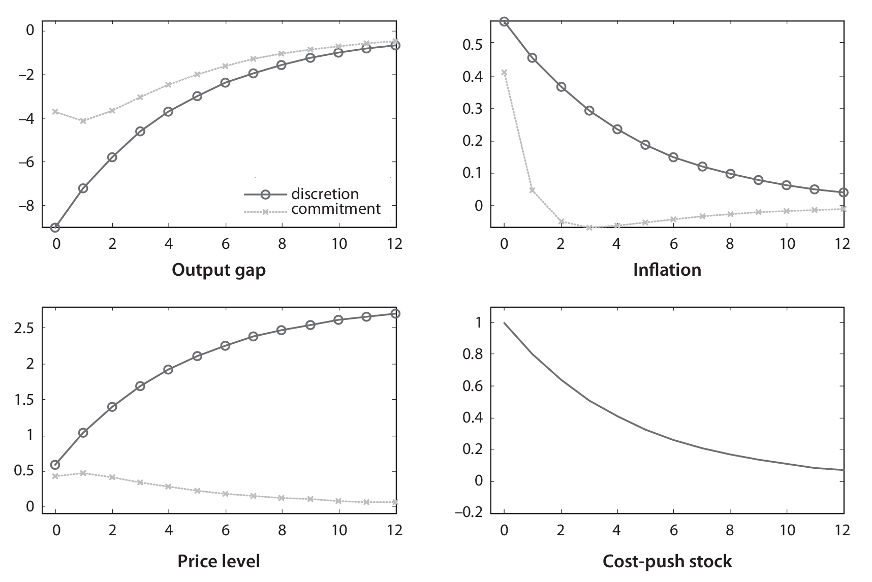
Optimal Monetary Policy below the Zero Lower Bound

Assume the optimal rule is: $i_t=r_t^n+{\varphi }_{\pi }{\pi }_t$ which shows that shocks to the natural rate (e.g., technology shocks) making the natural rate negative. In such case, it would be impossible to have zero inflation and zero output gap with a non-negative interest rate.

Assume that the natural rate has a steady state of 4% (quite unrealistic, these days) and has shock of -4% for 5 periods which is completely unanticipated and whose duration is known (perfect foresight). (A similar shock can be induced by manually imposing a decline in $z_t$) What would a central bank do?

If they act under discretion, the answer is intuitive and easy to formalize. The nominal rate drops to zero for the length of the shock; after period 6, output gap and inflation are at 0. The central bank under discretion wouldf want to lower below 0, but it cannot. Not surprisingly, the output gap and inflation are negative during the shock.

The central bank can improve under the commitment case. In fact, they can keep the interest rate at 0 for two extra periods. The main consequence is that output gap and inflation are much more stable. Thanks to the Dynamic IS equation, which depends on expected future interest rates, the central bank can afffect expectations and reduce the output loss, stimulating the economy.

A more detailed treatment of such cases can be found here.

Empirical Evidence on Interest Rate Rules

In recent times, central banks have adopted interest rate(s) as their main monetary policy tool. The literature on interest rate rules started with Taylor (1993), the original proposer of an interest rate rule thereafter known as the Taylor rule. Taylor proposed a formula that, in his view, was a good description of how the Fed set interest rate during Greenspan’s chairmanship (1987-1992). The formula appears as follows:

$$i_t^{(a)}=4.0+1.5\left({\pi }_t^{(4)}-2.0\right)+0.5{\hat{y}}_t$$

where the quarterly formula is obtained by dividing coefficients by 4 (apart from the response parameter 1.5 which is constant)

$$i_t=1.0+1.5({\pi }_t-0.5)+0.125{\hat{y}}_t$$

and ${\hat{y}}_t$ is the traditional output gap or detrended log GDP. To implement this rule in actual practice, the Fed injects or withdraws liquidity in the market to move interest rates towards the target by free market operations. The natural interpretation of 2.0 is as the inflation target over annual basis. The nominal rate should be around 2%, and 4.0 is the intercept consistent with an inflation target of 2% and such a natural rate.

Although Taylor was aiming at providing a purely positive account of practical policymaking, ex post many economists resolved to give it a normative interpretation. Great Moderation is a remarkable example. During the so-called Great Moderation, inflation was stable and low and recession were few and mild. As a consequence, a consensus arose that the Taylor rule was consistent with desirable macroeconomic outcomes: those experienced during the Great Moderation. Once this normative perspective is adopted, it is possible to evaluate monetary policy in historical periods or economies by comparing the interest rate set by the central bank at any point in time with that implied by the Taylor rule. Taylor did so in his 1999 paper, showing that from 1960 to 1986 the Taylor rule deviates hugely from actual practice, i.e. the historical Federal Funds Rate. In particular, the deviations were typically positive from 1960 to 1980, suggesting that monetary policy was too expansionary (i.e. the interest was too low) if we assume the Taylor rule as a normative benchmark. Taylor interprets this as one of the reasons why this period displayed high and volatile inflation and volative economic activity. At the end of the sample, the opposite is observed: the Federal Funds Rate were above the Taylor rate from 1979 to 1987. In fact, Paul Volker was appointed as chairman of the Fed in 1979, where he declared he would reduce inflation from 10% ca. through strong tightening of monetary policy. Taylor interprets this as the transition to lower levels of inflation, which required extra tightening to enforce central bank credibility. Since then, the Taylor rule performed relatively well, expect for periods where the zero lower bound was binding: there, the Taylor rule would call for negative funds rate, which could not be supported by the Fed.

In subsequent years, economists tried to estimate precise values for Taylor rules. For instance, in Clarida, Galì and Gertler (QJE 2000) the authors estimate a rule closer to the Fed’s actual policy:

$$i_t=\rho i_{t-1}+(1-\rho )[r+{\pi }^{\ast }+\beta {\mathbb{E}}_t[{\pi }_{t+1}-{\pi }^{\ast }]+\gamma {\mathbb{E}}_t[y_{t+1}-y_{t+1}^{\ast }]]$$

The main differences from the original Taylor rule are as follows. To begin with, adjustments are partial, which has become a standard for present central bank rules. That is to say, the central bank has some target for its interest rate, but the actual rate is adjusted gradually towards that. Moreover, the central bank does not respond to current values for inflation and output, but in anticipation to future values based on their forecasts. This is consistent with central bank releases about their policy choice. The rule was estimated with instrumental variables (the expectation is substituted by the actual value, which included the error term as th “surprise”, which is orthogonal to expectations under the rational expectations assumption and thus is exogenous). Splitting the sample in the pre-Volcker and the Volcker-Greenspan era, it is possible to see how parameters were dramatically shifted, in particular for the $\beta$ growing from 0.83 to 2.15.

If these estimates are taken seriously and embedded in the NK model, the condition for uniqueness of the equilibrium is, however, not satisfied during the pre-Volcker period. Thus, it allows the conjecture that the instability of the pre-Volcker period could be interpreted as the result of a molteplicity of equilibria, being subject to sunspot fluictuation. This is very different from the traditional hypothesis based on fundamentals, such as oil price shocks. Put simply, some fluctuations may be given by revisions of expectations that became self-fulfilling. For example, if agents assumed that inflation would be higher, and the central bank did not increase the nominal rate as much as it should, the real rate would have gone down, stimulating the economy and inducing self-fulfilling inflation. More formally, in the context of this example, suppose some variable follows any path of $x$ satisfying the following equation is an equilibrium:

$$x_t=\alpha {\mathbb{E}}_t[x_{t+1}]$$

For $|\alpha |>1$, this can be rewritten as

$${\mathbb{E}}_t[x_{t+1}]=\frac{1}{\alpha }{x}_t$$

which can be solved for stationary fluctuations of

$$x_{t+1}=\frac{1}{\alpha }{x}_t+{\xi }_{t+1}$$

leading to stationary sunspot equilibria.

Moving forward, Orphanides (JME 2003) made a very important point, which is by now very well understood. Put simply, when researchers estimate interest rate rules, they use data available to the researcher but not to the policymaker: the former operate ex post, while the latter makes forecasts ad interim. Thus, the author constructed real-time datasets including the values available to policymakers at each point in time (working at the Board of Governors of the Fed, he could access the Green Book which records the most recent estimates and forecasts of the central bank). It emerged that the real-time series related to the final series in a very imperfect way. In particular, in the case of the output gap, deviations were huge. Orphanides computed the interest rate imputed by the Taylor rule using the real-time series and concluded that the real-time series adhered to the Federal Funds Rate. The Fed was not doing the wrong thing: they were following the Taylor rule, but using ill-quality information. (What is starking is that policymakers would basically appear to be using a Taylor rule in the mid ’60s, before Taylor published his rule!) Why did Fed economists make such mistakes about output gaps? The likely answer lies in the notorious productivity slowdown: log-GDP in the post-war US had a clear shift in the trend during the 60s — indeed known as the productivity slowdown —, which was ultimately recovered during the 90s and until the GFC. Before the slowdown, output was fluctuating around a trend, and economists working at the Fed assumed that the previous trend would continue in present times. Thus, estimates of the output gap were becoming more and more negatively biased, until the productivity slowdown ultimately became to be captured by data analysis. This would be further grounded by the fact that predictions of inflation were actually on point. Orphanides concludes that there were no significant differences in the coefficients, but rather errors in real-time data. The Orphanides rule is thus based on nowcasting:

$$i_t=r+\pi +{\varphi }_{\pi }({\mathbb{E}}_t[{\pi }_t]-\pi )+{\varphi }_y{\mathbb{E}}_t[{\tilde{y}}_t]$$

and was updated in 2013 as:

$$\Delta i_t^{(a)}=0.5({\mathbb{E}}_t[{\pi }_{t+4}^{(4)}]-\pi )+0.5({\mathbb{E}}_t[\Delta y_{t+4}^{(4)}]-\Delta y_t^{\ast })$$

where ${\mathbb{E}}_t[{\pi }_{t+4}^{(4)}]$ is the expected inflation over the next four quarters on an annualized basis (note that this is using GDP change and not GDP gap: using GDP change makes the rule more robust, as gross mistakes such as those made by the Fed would be dodged). This is an example of first-difference rule, especially used in the central bank. They use the actual forecasts of professional forecasters to estimate an interval for inflation, and thereby compute an envelope of prescriptions for their simple policy rule, leading to a very good fit with actual data.

Sticky Wages and Unemployment in the New Keynesian Model

In the previous models, it was assumed that labor markets were competitive:

$$w_t-p_t=mr{s}_t$$

For instance, competitiveness in labor markets was implicit in the derivation of the optimality conditions inasmuch as households could supply labor without quantity constraints. From the standpoint of firms, competitiveness was also assumed in that firms could hire labor only at the market wage, where both sides were taking wages as given. In contrast, imperfections in the labor markets will be introduced in this chapter. In particular, the assumption of perfect competition in the labor market is dropped. There are several ways to deviate from perfect competition. A very generic specification may be proposed by defining the gap between the market rate of substitution and the real wage:

$$w_t-p_t={\mu }_t^w+mr{s}_t$$

where ${\text{mrs}}_t=\sigma c_t+\varphi n_t$ from the household’s optimality conditions. This wedge will be referred to as the (log) wage markup, the markup of the wage over the rate of substitution in the same way that the price markup was the wedge between actual price and its correspondent in perfect competition. Assume that the markup gap is non-negative (quite unpleasantly, a negative wage markup would suggest that workers are forced to work). Empirically speaking, sources of wage markup may lie in:

• efficiency wages: firms set wages at a higher level than the competitive wage hoping to induce higher (unobservable) effort by workers
• minimum wages
• workers’ market power (frictions, unions, search and matching models), usually implying positive wage markups In particular, however, our focus will not involve the existence of wage markups; whatever their source, we will take their existence for granted and rather focus on the variations in wage markups, and the attending effect on economic activity.

A main source of variations in wage markups will lie in sticky wages, in the same way as the price markup was affected by sticky prices. Nominal wages are non adjusted continuously, as highlighted by a large body of evidence. The distribution of individual wage changes shows that wages are not adjusted for a large fraction of workers.

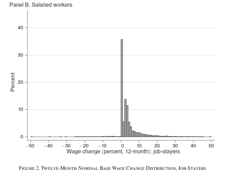
Similarly, the WDN survey (wage dynamics survey) contained in the WDN Final Report (2019) suggests that only a small fraction of workers has their wage adjusted more frequently than once a year, with a majority of workers adjusting every year and a significant fraction which adjusts even less frequently.

Sticky Wages and Inflation Dynamics

With sticky wages, wage inflation will also be part of the inflation dynamics picture. Recall that inflation was expressed in terms of the price markup gap, where this followed without any specific assumptions on labor market (or other externalities). Let us enrich the picture and assume for simplicity a production function linear in labor, so that the marginal productivity of labor is constant and equal to $A_t$ or in logs $a_t$ (the nominal marginal cost is thus $\frac{W_t}{A_t}$):

$$\begin{array}{rl}{\mu }_t^p& =p_t-(w_t-a_t)\\ & =a_t-{\omega }_t\\ & =a_t-({\mu }_t^w+\sigma c_t+\varphi n_t)\\ & =(1+\varphi )a_t-(\sigma +\varphi )y_t-{\mu }_t^w\end{array}$$

where ${\omega }_t=w_t-p_t$. Under the assumption of flexible prices and flexible wages, markups would be constant both for prices and wages: exploit this assumption to define natural levels of the markups and compute their deviations therefrom:

$${\mu }_t^p-{\mu }^p=-(\sigma +\varphi ){\tilde{y}}_t-({\mu }_t^w-{\mu }^w)$$

which ultimately allows to redefined a new implied NKPC:

$$\begin{array}{rl}{\pi }_t^p& =\beta {\mathbb{E}}_t[{\pi }_{t+1}^p]-{\lambda }_p({\mu }_t^p-{\mu }^p)\\ & =\beta {\mathbb{E}}_t[{\pi }_{t+1}^p]+{\lambda }_p[(\sigma +\varphi ){\tilde{y}}_t+{\mu }_t^w-{\mu }^w]\\ & =\beta {\mathbb{E}}_t[{\pi }_{t+1}^p]+{\kappa }_p{\tilde{y}}_t+{\lambda }_p{\hat{\mu }}_t^w\end{array}$$

where ${\lambda }_p\equiv \frac{(1-\theta )(1-\beta \theta )}{\theta }\Theta$ and ${\kappa }_p\equiv \left(\sigma +\varphi \right){\lambda }_p$, in analogy with the parameter $\kappa$ in the benchmark Phillips curve assuming that $\alpha =0$, that is $\kappa \equiv \left(\sigma +\frac{\varphi +\alpha }{1-\alpha }\right)\lambda$. This highlights a tradeoff between inflation and output gap stabilization. The Divine Coincidence result previously derived gets basically lost once wage markups are introduced. In addition, note that this source of inefficiency differs from the cost-push shock NKPC: the cost push involved a difference between natural and efficient levels of output, which could very much coincide in this case. Moreover, cost push is exogenous to monetary policy, whereas in general monetary policy will be able to affect the wage markup.

A Model with Sticky Wages and Prices

Original reference: Erceg-Henderson-Levin (JME 2000).

The key assumptions in this model, which is built upon the NK model, includes differentiated labor services, which can be interpreted as various “occupations”. Each occupation is represented by a union, with some specific market power when setting the wage, facing a labor demand schedule in the same way as firms face a demand for their good. Lastly, in analogy to price setting, nominal wage setting will also be staggered with constant probability $1-{\theta }_w$.

The representative household’s problem involves the term $\{{\mathcal{N}}_{t(j)}\}$: that is, each household includes individuals specialized in some specific labor service(s) $j$. Labor income will thus be equal to ${\int }_0^1{W}_t(j){\mathcal{N}}_t(j)dj$. This induces a difference in budget constraints and utility functions:

$$U(C_t,\{{\mathcal{N}}_t(j)\},Z_t)=\{\begin{array}{ll}\left(\frac{C_t^{1-\sigma }-1}{1-\sigma }-{\int }_0^1\frac{{\mathcal{N}}_t(j{)}^{1+\varphi }}{1+\varphi }dj+{\Xi }_t^{\sigma }\frac{L_t^{1-\sigma }-1}{1-\sigma }\right)Z_t& \sigma \ne 1\\ \left(\log (C_t)-{\int }_0^1\frac{{\mathcal{N}}_t(j{)}^{1+\varphi }}{1+\varphi }dj+{\Xi }_t^{\sigma }\log (L_t)\right)Z_t& \sigma =1\end{array}$$

where $\{{\mathcal{N}}_t(j)\}$ taken as given and $\log (Z_t)\equiv z_t\sim$ AR(1): this implies that the intratemporal optimality condition disappears. In contrast, the optimality conditions simply become:

$$Q_t=\beta {\mathbb{E}}_t\left[\left({\frac{C_{t+1}}{C_t}}^{-\sigma }\right)\left(\frac{Z_{t+1}}{Z_t}\right)\left(\frac{P_t}{P_{t+1}}\right)\right]$$

and its log-linearized counterpart:

$$c_t={\mathbb{E}}_t[c_{t+1}]-\frac{1}{\sigma }(i_t-{\mathbb{E}}_t[{\pi }_{t+1}^p]-\rho )+\frac{1}{\sigma }(1-{\rho }_z)z_t$$

The novelty of this model lies in wage setting. At each period $t$, a fraction $1-{\theta }_w$ of the unions renegotiates the wage following an optimal resetting rule:

$$\underset{W_t^{\ast }}{\max }{\mathbb{E}}_t\left[\sum _{k=0}^{\infty }(\beta {\theta }_w{)}^k\left(C_{t+k}^{-\sigma }\frac{W_t^{\ast }}{P_{t+k}}{N}_{t+k|t}-\frac{N_{t+k|t}^{1+\varphi }}{1+\varphi }\right)Z_{t+k}\right]$$

subject to the labor demand schedule (which will be derived below):

$$N_{t+k|t}={\left(\frac{W_t^{\ast }}{W_{t+k}}\right)}^{-{ϵ}_w}{N}_t$$

where $W_t\equiv {\left({\int }_0^1{W}_t(j{)}^{1-{ϵ}_w}dj\right)}^{\frac{1}{1-{ϵ}_w}}$. Note that:

$$\begin{array}{rl}{N}_{t+k|t}& ={\left(\frac{W_t^{\ast }}{W_{t+k}}\right)}^{-{ϵ}_w}{N}_t\\ & =(W_t^{\ast }{)}^{-{ϵ}_w}(W_{t+k}{)}^{{ϵ}_w}{N}_t\\ \frac{\partial N_{t+k|t}}{\partial W_t^{\ast }}& =\frac{\partial }{\partial W_t^{\ast }}\left[(W_t^{\ast }{)}^{-{ϵ}_w}(W_{t+k}{)}^{{ϵ}_w}{N}_t\right]\\ & =-{ϵ}_w(W_t^{\ast }{)}^{-{ϵ}_w-1}(W_{t+k}{)}^{{ϵ}_w}{N}_t\\ & =-{ϵ}_w(W_t^{\ast }{)}^{-{ϵ}_w-1}\left(N_{t+k|t}(W_t^{\ast }{)}^{{ϵ}_w}\right)\\ & =-{ϵ}_w(W_t^{\ast }{)}^{-{ϵ}_w-1+{ϵ}_w}{N}_{t+k|t}\\ & =-{ϵ}_w(W_t^{\ast }{)}^{-1}{N}_{t+k|t}\\ & =-{ϵ}_w\frac{N_{t+k|t}}{W_t^{\ast }}\end{array}$$

This is needed to derived the FOC applying the chain rule. The associated FOC can be found searching for the optimal labor supply of the household provided that the wage is resettled at time $t$. At each time $t+k$, it must hold that:

$$\begin{array}{rl}{\mathbb{E}}_t\left[\frac{\partial }{\partial W_t^{\ast }}\left(C_{t+k}^{-\sigma }\frac{W_t^{\ast }}{P_{t+k}}{N}_{t+k|t}-\frac{N_{t+k|t}^{1+\varphi }}{1+\varphi }\right)Z_{t+k}\right]& =0\\ {\mathbb{E}}_t\left[\left(\frac{C_{t+k}^{-\sigma }}{P_{t+k}}\left(N_{t+k|t}-{ϵ}_w{N}_{t+k|t}\right)-\left(N_{t+k|t}^{\varphi }\left(-{ϵ}_w\frac{N_{t+k|t}}{W^{\ast }}\right)\right)\right)Z_{t+k}\right]& =0\\ {\mathbb{E}}_t\left[\left(\frac{C_{t+k}^{-\sigma }}{P_{t+k}}{N}_{t+k|t}(1-{ϵ}_w)+{ϵ}_w\frac{N_{t+k|t}^{1+\varphi }}{W^{\ast }}\right)Z_{t+k}\right]& =0\end{array}$$

where the second line expands the product rule (left-hand term) and the chain rule (right-hand term). Let $U_{c,t+k}=C_{t+k}^{-\sigma }{Z}_{t+k}$ and $MR{S}_{t+k|t}=C_{t+k}^{\sigma }{N}_{t+k|t}^{\varphi }$, which implies $N_{t+k|t}^{\varphi }{Z}_{t+k}=MR{S}_{t+k|t}{C}_{t+k}^{-\sigma }{Z}_{t+k}=MR{S}_{t+k|t}{U}_{c,t+k}$. Then:

$$\begin{array}{rl}{\mathbb{E}}_t\left[U_{c,t+k}\frac{N_{t+k|t}}{P_{t+k}}\frac{{ϵ}_w}{{\mathcal{M}}_w}+{ϵ}_w\frac{N_{t+k|t}MR{S}_{t+k|t}{U}_{c,t+k}}{W_t^{\ast }}\right]& =0\\ {\mathbb{E}}_t\left[\frac{N_{t+k|t}{U}_{c,t+k}}{W_t^{\ast }}\left(\frac{{ϵ}_w}{{\mathcal{M}}_w}\frac{W_t^{\ast }}{P_{t+k}}+{ϵ}_{w}MR{S}_{t+k|t}\right)\right]& =0\\ {\mathbb{E}}_t\left[\frac{N_{t+k|t}{U}_{c,t+k}{ϵ}_w}{W_t^{\ast }}\left(MR{S}_{t+k|t}-\frac{1}{{\mathcal{M}}_w}\frac{W_t^{\ast }}{P_{t+k}}\right)\right]& =0\\ {\mathbb{E}}_t\left[\frac{N_{t+k|t}{U}_{c,t+k}}{W_t^{\ast }}\left(MR{S}_{t+k|t}-\frac{1}{{\mathcal{M}}_w}\frac{W_t^{\ast }}{P_{t+k}}\right)\right]& =0\\ {\mathbb{E}}_t\left[\frac{N_{t+k|t}{U}_{c,t+k}}{W_t^{\ast }}\left(\frac{W_t^{\ast }}{P_{t+k}}-{\mathcal{M}}_{w}MR{S}_{t+k|t}\right)\right]& =0\\ {\mathbb{E}}_t\left[N_{t+k|t}{C}_{t+k}^{-\sigma }{Z}_{t+k}\left(\frac{W_t^{\ast }}{P_{t+k}}-{\mathcal{M}}_{w}MR{S}_{t+k|t}\right)\right]& =0\end{array}$$

where ${ϵ}_w$ and $W_t^{\ast }$ could be taken out of the expectation since the former is a constant and the latter is known (and indeed, set) at time $t$. Put simply, the union maximizes the contribution that each occupation makes to the household — the easiest way to define and implement this objective function. This is given by the employment of such occupation in period $t+k$ times the corresponding wage. Putting together all the future streams of FOCs:

$$\sum _{k=0}^{\infty }(\beta {\theta }_w{)}^k{\mathbb{E}}_t\left[N_{t+k|t}{C}_{t+k}^{-\sigma }{Z}_{t+k}\left(\frac{W_t^{\ast }}{P_{t+k}}-{\mathcal{M}}_{w}MR{S}_{t+k|t}\right)\right]=0$$

Our ultimate goal is to derive a function which, given employment (set by firms) and a marginal rate of substitution, defines how the wage behaves. This differs from perfect competition, where wage was fixed and workers defined their own labor supply.

As an alternative solution method⁴, solve the wage-setting equation assuming flexible wages and deriving the first order conditions with respect to $W_t(i)$, imposing the constraint only afterwards:

$$\begin{array}{rl}\frac{C_t^{-\sigma }}{P_t}\left[N_t(j)+W_t(j)\frac{d{N}_t(j)}{d{W}_t(j)}\right]-N_t(j{)}^{\varphi }\frac{d{N}_t(j)}{d{W}_t(j)}& =0\\ & \\ \frac{C_t^{-\sigma }}{P_t}\left[1+\frac{W_t(j)}{N_t(j)}\underset{-{ϵ}_w}{\underbrace{\frac{d{N}_t(j)}{d{W}_t(j)}\frac{W_t(j)}{N_t(j)}}}\right]-\underset{-{ϵ}_w}{\underbrace{\frac{d{N}_t(j)}{d{W}_t(j)}\frac{W_t(j)}{N_t(j)}}}& =0\\ \frac{W_t(j)}{P_t}(1-{ϵ}_w)+C_t^{\sigma }{N}_t^{\varphi }(j){ϵ}_w& =0\\ & \\ w_t^{\ast }-p_t& ={\mu }_t^w+\sigma c_t+\varphi n_t(j)\end{array}$$

Plug this solution into the stream of profits and, in a way analogous to the baseline case, define the following objects:

$$\begin{array}{rl}{w}_t(j)& ={\mu }_w+mr{s}_t(j)+p_t\\ mr{s}_{t+k}& =\sigma c_{t+k}+\varphi n_{t+k}\\ mr{s}_{t+k|t}& =\sigma c_{t+k}+\varphi n_{t+k|t}\end{array}$$

To find the equation for the optimal wage, log-linearizing the term $\left(\frac{W_t^{\ast }}{P_{t+k}}-{\mathcal{M}}_{w}MR{S}_{t+k|t}\right)$ around the steady state where it is zero gives $\approx \overline{\left(\frac{W}{P}\right)}\left[(w_t^{\ast }-\bar{w})-(p_{t+k}-\bar{p})-({\mu }_w-{\bar{\mu }}_w)-(mr{s}_{t+k|t}-\overline{mrs})\right]$ . Ultimately, the equation for the optimal wage looks familiar.

$$\begin{array}{rl}0& =\sum _{k=0}^{\infty }(\beta {\theta }_w{)}^k{\mathbb{E}}_t\left[(w_t^{\ast }-\bar{w})-(p_{t+k}-\bar{p})-(mr{s}_{t+k|t}-\overline{mrs})\right]\\ w_t^{\ast }-\bar{w}& =(1-\beta {\theta }_w)\sum _{k=0}^{\infty }(\beta {\theta }_w{)}^k{\mathbb{E}}_t\left[(p_{t+k}-\bar{p})+(mr{s}_{t+k|t}-\overline{mrs})\right]\\ & =(1-\beta {\theta }_w)\sum _{k=0}^{\infty }(\beta {\theta }_w{)}^k{\mathbb{E}}_t[p_{t+k}+mr{s}_{t+k|t}]-(1-\beta {\theta }_w)\sum _{k=0}^{\infty }(\beta {\theta }_w{)}^k(\bar{p}+\overline{mrs})\\ & =(1-\beta {\theta }_w)\sum _{k=0}^{\infty }(\beta {\theta }_w{)}^k{\mathbb{E}}_t[p_{t+k}+mr{s}_{t+k|t}]-(\bar{p}+\overline{mrs})\\ w_t^{\ast }-({\mu }_w+\bar{p}+\overline{mrs})& =(1-\beta {\theta }_w)\sum _{k=0}^{\infty }(\beta {\theta }_w{)}^k{\mathbb{E}}_t[p_{t+k}+mr{s}_{t+k|t}]-(\bar{p}+\overline{mrs})\\ w_t^{\ast }& ={\mu }_w+\bar{p}+\overline{mrs}-(\bar{p}+\overline{mrs})+(1-\beta {\theta }_w)\sum _{k=0}^{\infty }(\beta {\theta }_w{)}^k{\mathbb{E}}_t[p_{t+k}+mr{s}_{t+k|t}]\\ w_t^{\ast }& ={\mu }_w+(1-\beta {\theta }_w)\sum _{k=0}^{\infty }(\beta {\theta }_w{)}^k{\mathbb{E}}_t[p_{t+k}+mr{s}_{t+k|t}]\end{array}$$

where ${\mu }^w=\log ({\mathcal{M}}_w)$ and ${\mathcal{M}}_w=\frac{{ϵ}_w}{{ϵ}_w-1}$ and $mr{s}_{t+k|t}\equiv \sigma c_{t+k}+\varphi n_{t+k|t}$. The optimal wage is forward looking: if prices or the marginal rate of substitution are expected to increase, the union recognizes that prices can be updated only occasionally and thus takes advantage of their reset time to impose a higher wage. Together with the wage setting rule, the usual wage dynamics hold, that is $w_t={\theta }_w{w}_{t-1}+(1-{\theta }_w)w_t^{\ast }$, as well as the NKPC analogous, the wage inflation equation:

$${\pi }_t^w=\beta {\mathbb{E}}_t[{\pi }_{t+1}^w]-{\lambda }_w({\mu }_t^w-{\mu }^w)$$

where ${\lambda }_w\equiv \frac{(1-\beta {\theta }_w)(1-{\theta }_w)}{{\theta }_w(1+\varphi {ϵ}_w)}$.

As in the basic NK model, firms produce a final good with technology $Y_t(i)=A_t{N}_t(i{)}^{1-\alpha }$ and $\log A_t\equiv a_t\sim$ AR(1). However, there is an effective labor input index, which involves the integration of the types of labor services under CES assumption:

$$N_t(i)={\left({\int }_0^1{N}_t(i,j{)}^{\frac{e_w-1}{e_w}}dj\right)}^{\frac{{ϵ}_w}{{ϵ}_w-1}}$$

A firm maximizing profits will, in a first stage, choose optimally the composition and quantities of the labor services, for any given level of the effective labor input. That is, taking $N_t(i)$ as given for any level of $N_t(i)$, the cost minimization occurs at:

$$N_t(i,j)={\left(\frac{W_t(j)}{W_t}\right)}^{-{ϵ}_w}{N}_t(i)$$

The implication is that the cost for the firm is equal to the wage index weighted by their composition of labor:

$${\int }_0^1{W}_t(j)N_t(i,j)dj=W_t{N}_t(i)$$

while the rest of the derivation for the firm problem is the same as in the baseline model. Price setting also works in the same way as in the benchmark NK model.

Equilibrium

As usual, markets clear in equilibrium. For the final good market, this means $Y_t=C_t$. Let us turn to the labor market. Aggregate employment is obtained by aggregating hours of work from all firms and occupations. The goal is to write as a function of aggregate output:

$$\begin{array}{rl}{N}_t& \equiv {\int }_0^1{\int }_0^1{N}_t(i,j)djdi\\ & \\ & ={\int }_0^1{N}_t(i){\int }_0^1\frac{N_t(i,j)}{N_t(i)}djdi\\ & ={\Delta }_{w,t}{\int }_0^1{N}_t(i)di\\ & ={\Delta }_{w,t}{\left(\frac{Y_t}{A_t}\right)}^{\frac{1}{1-\alpha }}{\int }_0^1{\left(\frac{Y_t(i)}{Y_t}\right)}^{\frac{1}{1-\alpha }}di\\ & ={\Delta }_{w,t}{\Delta }_{p,t}{\left(\frac{Y_t}{A_t}\right)}^{\frac{1}{1-\alpha }}\end{array}$$

where the $\Delta$ are indices of wage and price dispersion.

$$\{\begin{array}{l}{\Delta }_{w,t}\equiv {\int }_0^1{\left(\frac{W_t(j)}{W_t}\right)}^{-{ϵ}_w}dj\\ {\Delta }_{p,t}\equiv {\int }_0^1{\left(\frac{P_t(i)}{P_t}\right)}^{\frac{-{ϵ}_p}{1-\alpha }}di\end{array}$$

which implies that the following relation between aggregate output and aggregate employment holds:

$$(1-\alpha )n_t=y_t-a_t+d_{w,t}+d_{p,t}$$

where $d_{w,t}\equiv \log \left[{\int }_0^1{\left(\frac{W_t(j)}{W_t}\right)}^{-{ϵ}_w}\right]$ and $d_{p,t}\equiv \log \left[{\int }_0^1{\left(\frac{P_t(i)}{P_t}\right)}^{\frac{-{ϵ}_p}{1-\alpha }}\right]$. As shown in the derivation of price dispersion, these are approximately equal to $\frac{{ϵ}_p}{2\Theta }\text{var}(p_t(i))$ (which is exactly the same derivation) and $\frac{(1-\alpha ){ϵ}_w}{2}{\text{var}}_j(w_t(i))$ (a similar argument). Up to a first order approximation, it holds that:

$$(1-\alpha )n_t=y_t-a_t$$

As we will see, this is the mechanism behind the losses for price inflation and wage inflation.

To find a new version of the equations for price and wage inflation, note that the output gap is based on natural output, which should now be understood with reference to equilibrium levels of both flexible prices and flexible wages. Let us define a new object, the wage gap:

Wage Gap

$${\tilde{\omega }}_t\equiv {\omega }_t-{\omega }_t^n$$

where ${\omega }_t\equiv w_t-p_t$ and ${\omega }_t^n$ is the natural real wage (determined below).

$$\begin{array}{rl}{\omega }_t^n& =\log (1-\alpha )+(a_t-\alpha n_t^n)-{\mu }^p\\ & =\log (1-\alpha )+{\psi }_{wa}{a}_t-{\mu }^p\end{array}$$

with ${\psi }_{wa}\equiv \frac{1-\alpha {\psi }_{ya}}{1-\alpha }$ and ${\psi }_{ya}=\frac{1+\varphi }{\sigma (1-\alpha )+\varphi +\alpha }$ as in the NK model. The price markup gap can be derived, so as to obtain a new implied price inflation equation.

$$\begin{array}{rl}\{\begin{array}{ll}{\mu }_t^w& =\log (1-\alpha )+(a_t-\alpha n_t)-{\omega }_t\\ {\mu }^p& =\log (1-\alpha )+(a_t-\alpha n_t^n)-{\omega }_t^n\end{array}⟹{\hat{\mu }}_t^p& =(mp{n}_t-{\omega }_t)-{\mu }^p\\ & =({\tilde{y}}_t-{\tilde{n}}_t)-{\tilde{\omega }}_t\\ & =-\frac{\alpha }{1-\alpha }{\tilde{y}}_t-{\tilde{\omega }}_t\end{array}$$

The novelty is that price inflation will now depend also on the markup gap. In fact, the implied price inflation equation is as follows:

$${\pi }_t^p=\beta {\mathbb{E}}_t[p_{t+1}]+\varkappa {\tilde{y}}_t+{\lambda }_p{\tilde{\omega }}_t$$

where $\varkappa \equiv \frac{\alpha {\lambda }_p}{1-\alpha }$. Similarly, the wage markup gap will imply a new wage inflation equation. The markup gap results as:

$$\begin{array}{rl}{\hat{\mu }}_t^w& ={\omega }_t-{mrs}_t-{\mu }^w\\ & ={\tilde{\omega }}_t-(\sigma {\tilde{y}}_t+\varphi {\tilde{n}}_t)\\ & ={\tilde{\omega }}_t-\left(\sigma +\frac{\varphi }{1-\alpha }\right){\tilde{y}}_t\end{array}$$

And the wage inflation in terms of the output and real wage gaps:

$${\pi }_t^w=\beta {\mathbb{E}}_t[{\pi }_{t+1}^w]+{\varkappa }_w{\tilde{y}}_t-{\lambda }_w{\tilde{\omega }}_t$$

where ${\varkappa }_w\equiv {\lambda }_w\left(\sigma -\frac{\varphi }{1-\alpha }\right)$. In addition, there is an identity relating the changes in the wage gap to price inflation, wage inflation, and the natural wage:

$${\tilde{\omega }}_t\equiv {\tilde{\omega }}_{t-1}+{\pi }_t^w-{\pi }_t^p-\Delta {\omega }_t^n$$

In order to complete the nonpolicy block of the model, the previous equilibrium conditions (that is, ^ae3eed, ^68c52c and ^faca40 ) must be supplemented with a Dynamic IS equation similar to the previous and derived from the goods market clearing condition combined with the Euler ^c2650a:

$${\tilde{y}}_t=-\frac{1}{\sigma }(i_t-{\mathbb{E}}_t[{\pi }_{t+1}^p]-r_t^n)+{\mathbb{E}}_t[{\tilde{y}}_{t+1}]$$

which involves the natural interest rate $r_t^n\equiv \rho -\sigma (1-{\rho }_a){\psi }_{ya}{a}_t+(1-{\rho }_z)z_t$. Its derivation is similar to ^6083fa and should be interpreted as the prevailing real rate in an equilibrium with flexible wages and flexible prices. For a solution to the model, also assume that the interest rate follows the following simple rule:

$$i_t=\rho +{\varphi }_p{\pi }_t^p+{\varphi }_w{\pi }_t^w+{\varphi }_y{\hat{y}}_t+v_t$$

where $v_t$ is the usual exogenous component with zero mean. This can be plugged into ^89f626 so as to get rid of the interest rate. In a similar vein as in the benchmark model, represent this dynamic system in the following form:

$${\mathbf{A}}_0^w{\mathbf{x}}_t={\mathbf{A}}_1^w{\mathbb{E}}_t[{\mathbf{x}}_{t+1}]+{\mathbf{B}}_0^w{\mathbf{u}}_t$$

where ${\mathbf{x}}_t\equiv [{\tilde{y}}_t,{\pi }_t^p,{\pi }_t^w,{\tilde{\omega }}_{t-1}{]}^{⊺}$, ${\mathbf{u}}_t\equiv [{\hat{r}}_t^n-v_t-{\varphi }_t{\hat{y}}_t^n,\Delta {\omega }_t^n{]}^{⊺}$, and the matrices are:

$${\mathbf{A}}_0^w\equiv \left[\begin{array}{cccc}\sigma +{\varphi }_t& {\varphi }_p& {\varphi }_w& 0\\ -{\varkappa }_p& 1& 0& 0\\ -{\varkappa }_w& 0& 1& 0\\ 0& -1& 1& 1\end{array}\right]{\mathbf{A}}_1^w\equiv \left[\begin{array}{cccc}\sigma & 1& 0& 0\\ 0& \beta & 0& {\lambda }_p\\ 0& 0& \beta & {\lambda }_w\\ 0& 0& 0& 1\end{array}\right]{\mathbf{B}}_0^w\equiv \left[\begin{array}{cc}1& 0\\ 0& 0\\ 0& 0\\ 0& 1\end{array}\right]$$

Note that ^c33f84 may not have a solution satisfying ${\tilde{y}}_t={\pi }_t^p={\pi }_t^w=0$ at all points (details are excruciating and contained in the textbook). Moreover, local uniqueness that three eigenvalues lie inside and one eigenvalue lies outside the unit circle for the matrix ${\mathbf{A}}^w\equiv ({\mathbf{A}}_0^w{)}^{-1}{\mathbf{A}}_1^w$. The solution is:

$${\varphi }_p+{\varphi }_w+{\varphi }_y\left(\frac{1-\beta }{\sigma +\frac{\alpha +\varphi }{1-\alpha }}\right)\left(\frac{1}{{\lambda }_p}+\frac{1}{{\lambda }_w}\right)>1$$

which for ${\varphi }_y=0$ simplifies to ${\varphi }_p+{\varphi }_w>1$. The central bank must adjust the nominal rate more than one-for-one in response to variations in any arbitrary weighted average price and wage inflation.

Dynamic Responses to a Monetary Policy Shock

Assume a tightening of monetary policy, i.e. a positive realization of $v_t$. In all cases there is a recession, a persistent reduction in output, with the strongest response in the baseline case (with both sticky wages and prices), but similar patterns along the three.

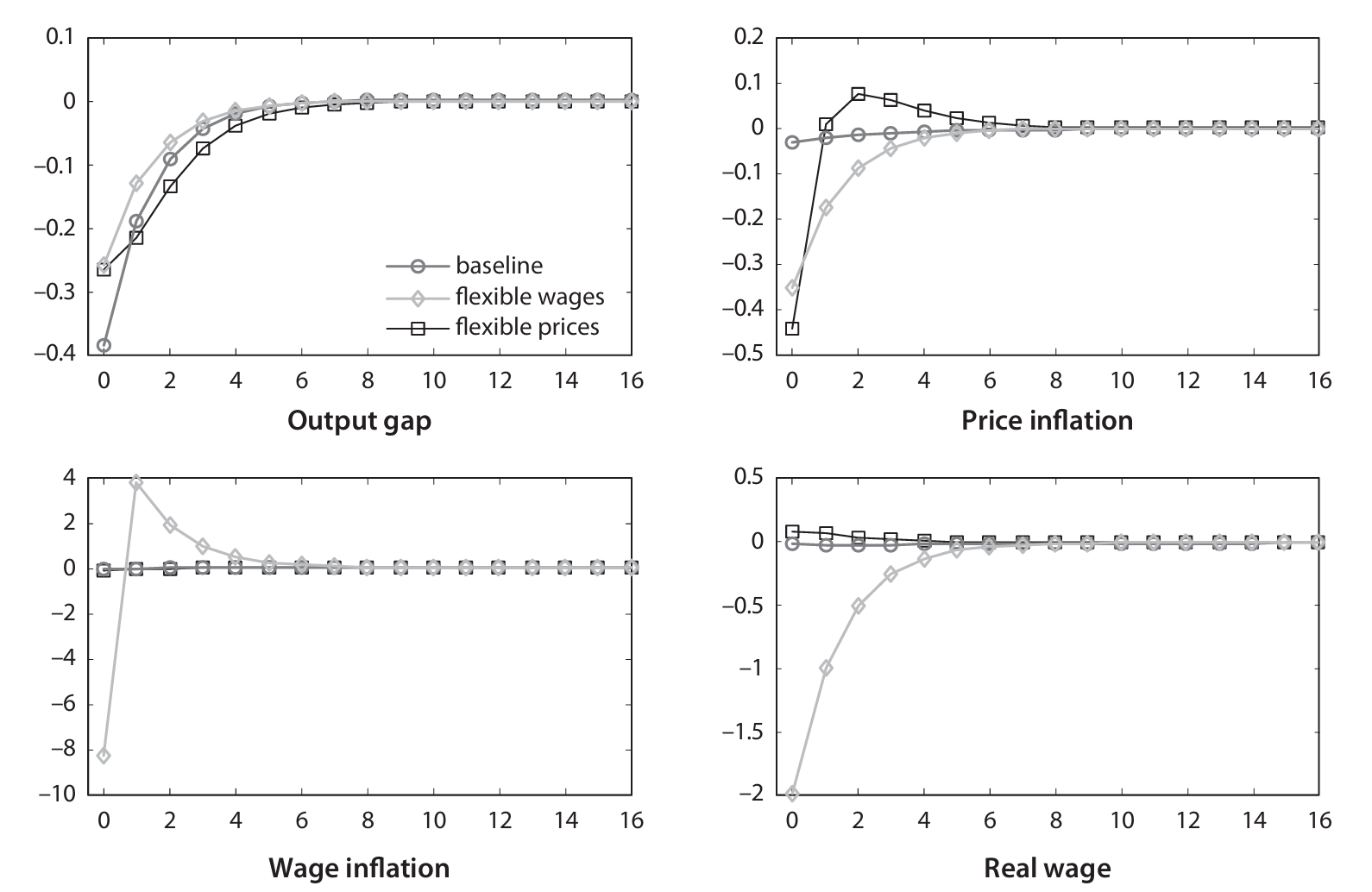
The main differences are, obviously, in the responses to price inflation and wage inflation. When prices are flexible, the decrease in price inflation is larger. Note that, in the baseline case, there is also no decline in price inflation. As for wage inflation, the largest responce obviously occurs when wages are flexible. Last, the response of the real wage is very different across models. In the baseline case, price and wage inflation hardly change… not surprisingly: in the baseline, both are sticky. Why do sticky wages reduce the response of price inflation? Why do they induce some additional endogenous stickyness in prices? Recall the optimal price setting conditions: firms set prices based on expected marginal costs. Sticky wages are an important component of marginal costs: firms will not respond so strongly if wages do not move and marginal costs do not soar. As for wages, unions reset wages based on current and expected marginal rates of substitution and, importantly, prices. If prices are sticky, then also the reset optimal wage becomes stickier. Combine the two, a positive feedback generates the reinforcement loop leading to the tiny responses of real wages and inflation in the simulated models.

Real wages also exhibit cyclical behavior. Depending on the models, they can be cyclical, procyclical, or countercyclical: this depends basically on the relative stickiness of wages and prices. An insightful connection with the history of economic thought can be sketched. A key message of The General Theory of Occupation, Interest, and Money is that fluctuations are basically driven by demand shocks. In Keynes’s framework, he was basically emphasizing sticky wages, assuming flexible prices. An implication of such a model is that the real wage is countercyclical, as the previous numerical simulations suggest. In response, a number of authors critized the General Theory on the grounds that real wages were, empirically, not countercyclical but rather procyclical. When the New Keynesian models emerged, the problem of the old Keynesian models was finally understood, leading NK authors to focus initially on price stickiness in particular: to get procyclical real wage, prices have to be sufficiently sticky relative to wages. Later on, however, especially as a result of the work by Blanchard and Kiyotaki, it became very clear that both prices and wages could be sticky, and any type of cyclicality could be generated with a suitable calibration of the relative rigidity of the two.

Dynamic Responses to a Technology Shock under the Optimal Monetary Policy

For simplicity, assume that the steady state is efficient. How can the steady state be efficient with monopolistic firms and labor unions market power? Implicitly, assumes that the inefficiencies introduced by market power are corrected by some instruments different than monetary policy. The easiest device is introducing a subsidy for unemployment. An example may be as follows:

$$\{\begin{array}{l}{P}_t={\mathcal{M}}_p\frac{W_t(1-\tau )}{MP{N}_t}⟹\Omega =\frac{MP{N}_t}{{\mathcal{M}}_p(1-\tau )}\\ \Omega ={\mathcal{M}}_{w}MRS\\ {\mathcal{M}}_p{\mathcal{M}}_w(1-\tau )MR{S}_t=MR{S}_t\end{array}$$

In order to make the steady state efficient, it must be that ${\mathcal{M}}_p{\mathcal{M}}_w(1-\tau )=1$.

Consider a second order approximation to the utility losses of the representative household with sticky prices and wages in an efficient steady state:

$$\min \frac{1}{2}{\mathbb{E}}_0\sum _{t=0}^{\infty }{\beta }^t\left[\left(\sigma +\frac{\varphi +\alpha }{1-\alpha }\right){\tilde{y}}^2+\frac{{ϵ}_p}{{\lambda }_p}({\pi }_t^p{)}^2+\frac{{ϵ}_w(1-\alpha )}{{\lambda }_w}({\pi }_t^w{)}^2\right]\text{ subject to }\{\begin{array}{ll}{\pi }_t^p& =\beta {\mathbb{E}}_t[{\pi }_{t+1}^w]+{\varkappa }_p{\tilde{y}}_t+{\lambda }_p{\tilde{\omega }}_t\\ {\pi }_t^w& =\beta {\mathbb{E}}_t[{\pi }_{t+1}^p]+{\varkappa }_w{\tilde{y}}_t+{\lambda }_w{\tilde{\omega }}_t\\ {\tilde{\omega }}_{t-1}& \equiv {\tilde{\omega }}_t-{\pi }_t^w+{\pi }_t^p+\Delta {\omega }_t^n\end{array}$$

This is equivalent to assuming that the natural equilibrium is efficient: in fact, once market power is corrected through the subsidy, then the natural equilibrium is efficient. In general, it is not feasible in this model to replicate the natural equilibrium, while it is feasible only under restrictive conditions. Still, suppose we replicate the natural equilibrium. Output gap would be 0, and thus also price inflation would be 0. Finally, wage inflation would also be 0 (both inflations at 0 is consistent with the desired markup realization). This forces the natural real wage to be constant (each of its addends would be 0), which is a very restrictive case. Thus, optimal policy is unlikely to follow the simple rule and stabilizing these variables altogether.

To solve for this, set up the Lagrangian with the three constraints and multipliers. Deriving the FOC and the derivative of the Lagrangian relative to the output gap, the following optimality conditions are obtained:

$$\{\begin{array}{l}\left(\sigma +\frac{\varphi +\alpha }{1-\alpha }\right){\tilde{y}}_t+{\varkappa }_p{\zeta }_{1,t}+\varkappa {\zeta }_{2,t}=0\\ \frac{{ϵ}_p}{{\lambda }_p}{\pi }_t^p-\Delta {\zeta }_{1,t}+{\zeta }_{3,t}=0\\ \frac{{ϵ}_w(1-\alpha )}{{\lambda }_w}{\pi }_t^w-\Delta {\zeta }_{1,t}-{\zeta }_{3,t}=0\end{array}$$

Keep in mind that, in equilibrium, the Lagrangian multipliers must be 0, and ${\tilde{\omega }}_{0-1}$ is given. This leads to a linear system of seven different equations including the Lagrangian multipliers (they cannot be eliminated as in the classical model). Rewrite the system in matrix form:

$${\mathbf{A}}_0^{\ast }{\mathbf{x}}_t={\mathbf{A}}_1^{\ast }{\mathbb{E}}_t[{\mathbf{x}}_{t+1}]+{\mathbf{B}}_0^{\ast }\Delta a_t$$

where ${\mathbf{x}}_t\equiv [{\tilde{y}}_t,{\pi }_t^p,{\pi }_t^w,{\tilde{\omega }}_{t-1},{\zeta }_{1,t-1},{\zeta }_{2,t-1},{\zeta }_{3,t}{]}^{⊺}$. The driving force lies in $\Delta {\omega }_t^n$, which explains why $\Delta a_t$ figures on the right hand side (?). The preference shock, instead, does not appear and remains implicit in the Dynamic IS equation. Annihilating the shocks:

$${\mathbf{A}}_0^{\ast }{\mathbf{x}}_t={\mathbf{A}}_1^{\ast }{\mathbb{E}}_t[{\mathbf{x}}_{t+1}]$$

With the additionall assumption that ${\tilde{\omega }}_{t-1}=0$, the solution to this system would be that $x_t=0$ for all $t$ (recall that the given starting value ${\omega }_{0-1}$ must also be 0 for this condition to be satisfied). To implement this, solve for the suitable nominal interest rate from the Dynamic IS equation:

$$i_t=r_t^n+{\varphi }_p{\pi }_t^p$$

where $r_t^n=\rho +(1-{\rho }_z)z_t$ and ${\varphi }_p>1$ leads to a unique solution to the difference equation in the vector $0$.

The optimal policy fully stabilizes output gap and inflations. With flexible prices and sticky wages can still replicate the natural equilibrium: price inflation jumps so that the real wage tracks the natural real wage. In formulae, this corresponds to ${\lambda }_p\to \infty$ in the minimization problem, so that price inflation doesn’t matter (in general, when prices are flexible, price inflation does not induce any welfare losses): prices take the burden of adjusting the real wage, in a costless way. In the baseline (sticky) calibration, the output gap exhibits a small deviation, with some negative price inflation and some positive wage inflation. This makes it possible for the real wage to increase very slightly: but far from matching the natural real wage, which would require a much larger positive (negative) wage (price) inflation.

It turns out that a policy that stabilizes the output gap in this model is not only approximately optimal. It is possible to show that for a particular calibration for parameter values is exactly optimal. But it is also true that a policy fully stabilizing the output gap is not far from the optimal policy. This has an interesting implication: In particular, a linear combination of the two Phillips curves would eliminate the wage gap, which is the problematic variable for policy purposes (being unobservable). In fact:

$$\begin{array}{c}\frac{{\lambda }_w}{{\lambda }_p+{\lambda }_w}{\pi }_t^p=\beta {\mathbb{E}}_t[\frac{{\lambda }_w}{{\lambda }_p+{\lambda }_w}{\pi }_{t+1}^p]+\frac{{\lambda }_w{\varkappa }_p}{{\lambda }_p+{\lambda }_w}{\tilde{y}}_t+\frac{{\lambda }_w{\lambda }_p}{{\lambda }_p+{\lambda }_w}{\tilde{\omega }}_t\\ \frac{{\lambda }_p}{{\lambda }_p+{\lambda }_w}{\pi }_t^w=\beta {\mathbb{E}}_t[\frac{{\lambda }_p}{{\lambda }_p+{\lambda }_w}{\pi }_{t+1}^p]+\frac{{\lambda }_p{\varkappa }_w}{{\lambda }_p+{\lambda }_w}{\tilde{y}}_t+\frac{{\lambda }_w{\lambda }_p}{{\lambda }_p+{\lambda }_w}{\tilde{\omega }}_t\\ {\pi }_t\equiv \frac{{\lambda }_w}{{\lambda }_p+{\lambda }_w}{\pi }_t^p+\frac{{\lambda }_p}{{\lambda }_p+{\lambda }_w}{\pi }_t^w\\ {\pi }_t=\beta {\mathbb{E}}_t[{\pi }_{t+1}]+\kappa {\tilde{y}}_t\end{array}$$

In this “composite” inflation, the Divine Coincidence holds back again: stabilizing output gap corresponds to stabilizing some weighted average of price inflation and wage inflation.

Unemployment

An alternative formulation of the model can highlight the role of unemployment rates into the model. The model is the same, and so will be all the equations described so far. There will be, however, an additional equation incorporating unemployment. Assume a representative household with a continuum of members employed in different sector: index the household as $(j,s)\in [0,1]\times [0,1]$, where $j$ is the labor sector. Moreover, assume that an individual is indivisible: either works (fully) or doesn’t work. The disutility from working is denoted as ${\xi }_t{s}^{\varphi }$ for $s\in [0,1]$ and $\varphi \ge 0$. The household fully share consumption risk, and their utility function is:

$${\mathbb{E}}_0\sum _{t=0}^{\infty }{\beta }^{t}U(C_t,\{{\mathcal{N}}_t(j)\};Z_t)$$

where the structural form of the utility function may be specified as:

$$\begin{array}{rl}U(C_t,\{{\mathcal{N}}_t(j)\};Z_t)& \equiv \left(\frac{C_t^{1-\sigma }-1}{1-\sigma }-\chi {\int }_0^1{\int }_0^{{\mathcal{N}}_t(j)}{s}^{\varphi }dsdj\right)\\ & =\left(\frac{C_t^{1-\sigma }-1}{1-\sigma }-\chi {\int }_0^1{\int }_0^{{\mathcal{N}}_t(j)}{\left[\frac{s^{1+\varphi }}{1+\varphi }\right]}_{s=0}^{s={\mathcal{N}}_t(j)}dj\right)\\ & =\left(\frac{C_t^{1-\sigma }-1}{1-\sigma }-\chi {\int }_0^1\frac{{\mathcal{N}}_t(j{)}^{1+\varphi }}{1+\varphi }dj\right)\end{array}$$

with optimality conditions similar to ^c2650a.

When does an individual participate in the labor market? Given the wage prevailing for their occupation, the utility brought to the household by a worker is the real wage times the utility generated to the household. This must be larger than their own disutility from working: $C_t^{-\sigma }\frac{W_t(j)}{P_t}\ge {\chi }_t{s}^{\varphi }$. The marginal participant in the labor market is that worker is sector $j$ such that $C_t^{-\sigma }\frac{W_t(j)}{P_t}={\chi }_t{L}_t(j{)}^{\varphi }$. Taking logs and integrating over $j$, this leads to the average wage:

$$w_t-p_t=\sigma c_t+\varphi l_t+{\xi }_t$$

where $w_t\equiv {\int }_0^1{w}_t(j)dj$ and the log labor force $l_t\equiv {\int }_0^1{l}_t(j)dx$ with ${\xi }_t=\log ({\chi }_t)$. Last, define th unemployment rate as $u_t\equiv l_t-n_t\approx \frac{L_t-N_t}{N_t}$. Note that this is not the way official statistics measure unemployment, which is rather equal to $\frac{L_t-N_t}{L_t}$ (the two are still similar for small values).

Define unemployment as $u_t\equiv l_t-n_t$. Based on the average markup, obtain:

$$\begin{array}{rl}{\mu }_t^w& =(w_t-p_t)-(\sigma c_t+\varphi n_t+{\xi }_t)\\ & =\varphi u_t\end{array}$$

where an unemployment similar to that computed by national agencies is proportional to the wage markup.

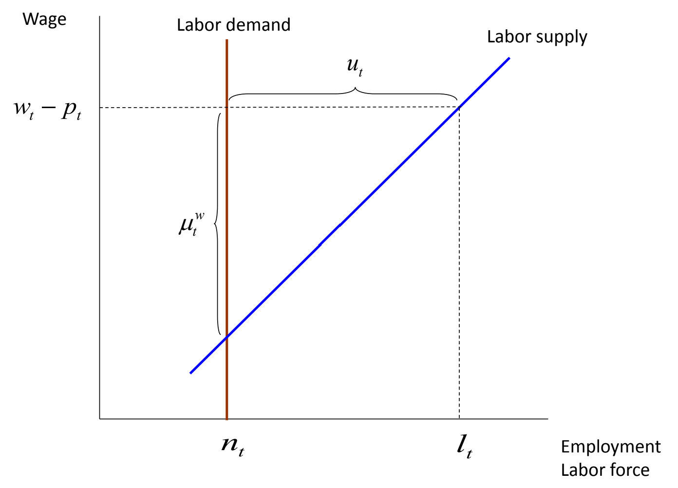
In this framework, define the natural rate of unemployment as the unemployment observed in equilibrium if wages were flexible: ${\mu }^w=\varphi u^n$. Therefore:

$${\mu }_t^w-{\mu }^w=\varphi (u_t-u^n)$$

This allows to rewrite the NKWPC in terms of unemployment:

$${\pi }_t^w=\beta {\mathbb{E}}_t[{\pi }_{t+1}^w]-{\lambda }_w\varphi (u_t-u^n)$$

This connects to the original Phillips Curve proposed by Phillips, which related wage inflation and unemployment. The stickier the wages, the smaller ${\lambda }_w$, and inflation responds less to unemployment.

Dynamic Response of Labor Market Variables to a Monetary Policy Shocks

The new equations allow to see how labor market variables react to a tightening of monetary policy (policy realization of $v_t$).

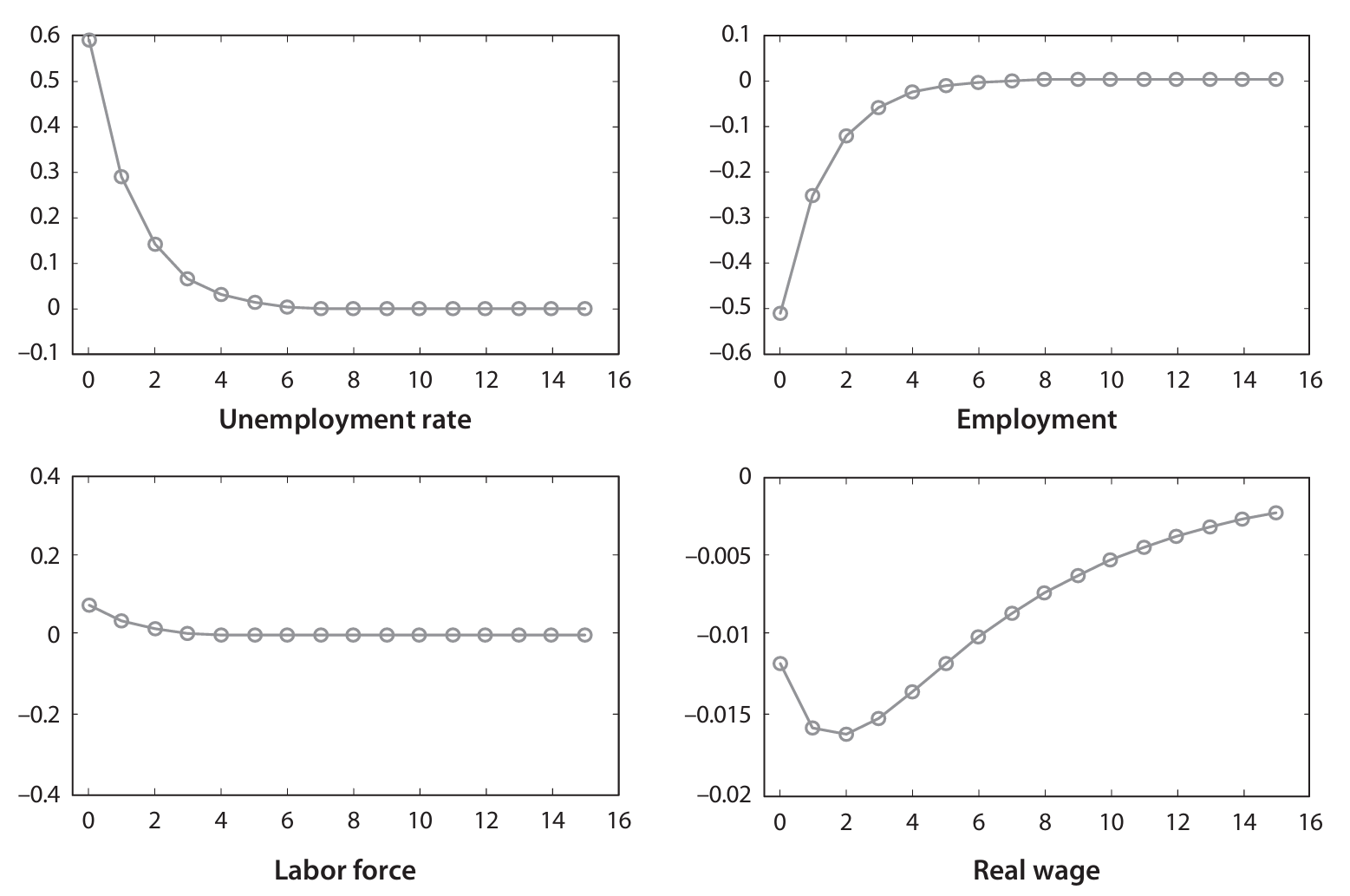
The unemployment rate decreasesm together with the real wage, with a slight increase in the labor force. Unemployment rate decreases more than employment, as the labor force is slightly increasing, due to the wealth effect of labor supply: consumption decreases, the marginal utility of consumption is higher, and a stronger incentive to work kicks in. If this were the only shock, it would imply countercyclical labor force: however, the data suggest that labor force is quite stable, and if it exhibits any cyclicality it would be procyclical. This issue is grappled with by Galì, Smets & Wauters, based on the Smets & Wauters model — a medium scale NK model, extended so as to incorporate investment, indexation, and other variables. In Galì, Smets and Wauters, unemployment is introduced and the model is taken to the data. In particular, it implements the ideas paper by Jaimovich and Rebelo, which modifies preferences to dampen labor supply shocks in the short run, into the Smauts and Wauters model. The labor supply equation would look thereby as:

$$p_t={\mu }^w+x_t+\varphi l_t+{\xi }_t$$

where $x_t\equiv \gamma x_{t-1}+(1-\gamma )c_t$. If $\gamma$ is large, $x_t$ would not change much, so that the wealth effect would not be completely eliminated but dampened. In the long run, however, $l_t$ would adjust, and $x_t$ and $c_t$ would identify. This would be consistent with balanced growth ($\sigma =1$) on the long run.

Conclusion: The New Keynesian Perspective on Economic Fluctuations

How to think to the NK model in a graphical way? Imagine a diagram with employment and wage, and assume that the real wage adjusts to the employment level (the Neoclassical Perspective). Empirical evidence will likely be at odds with such an economy. Suppose now to allow with “wedges”: the price and wage markups. It is possible to define the gap between marginal rate of substitution and marginal product of labor:

$$\begin{array}{rl}{\text{gap}}_t& \equiv mr{s}_t-mp{n}_t\\ & =-({\mu }_t^p+{\mu }_t^w)\le 0\end{array}$$

which is the Efficiency Gap: 0 is perfect competition, and the lower the gap, the greater the distortion (positive values would be possible only with firms selling below the production cost or workers working below their marginal disutility). In the Neoclassical Benchmark, then, it is possible to be everywhere in the area below the two schedules, and the gap is uniquely identified by the wage and price markups. A model is, however, needed to track the exact location of the real wage and the markups in that area. The NK model is one such model (for example, models with endogenous markups also exist). In this model, monopolistic competition in goods and labor markets induces positive desired markups, but sticky prices and wages allow for markups to fluctuate around their desired value (“elastic markups”). In fact, the desired markups allow to draw additional schedules. If we simply had a natural equilibrium (markups, but flexible prices), these new two schedules would determine the level of employment, namely below the centralized solution manner, and thus pin down output (natural equilibrium). Monetary policy would thus be neutral. With stickiness, however, markups can move around the intersection of such new schedules, so far as the non-negative markup regions is not violated. Whether the current real wage is above or below such intersection depends on the markup gaps, and in particular which one is positive and which one is negative. Monetary policy is no longer neutral. The greatest difference from the neoclassical perspective is that aggregate demand now finds its way in affecting the economy. A shock has some impact on aggregate demand, if the interest rate remains unchanged. However, an active monetary policy rule can affect the real interest rate, and work with aggregate demand to dampen or sustain a shock. In equilibrium, this is possible precisely thanks to elastic markups. Suppose only sticky prices where there: the wage markup would be constant and thus we would move only along the $mr{s}_{+}{\mu }^w$ schedule (and viceversa, along the $mpn-{\mu }^p$ is only sticky wages were there).

Footnotes

1. Note that the money demand equation has been derived assuming that the elasticity of real balances demand follows the same parameter as the elasticity of consumption. ↩

2. Assuming equilibrium, $C_t=Y_t$ and thus $Y_t(i)={\left(\frac{P_t(i)}{P_t}\right)}^{-ϵ}{Y}_t$. Taking logs yields the results desired. ↩

3. This is the only explanation I could come up with for the disappearance of the term $1+z_t$, provided that the math is correct. This derivation may be subject to revision later on. ↩

4. Namely, this is the “variational” solution method proposed during the lecture. ↩