Advanced Macroeconomics III (Jeenas)

Introduction

This final part of the course involves financial frictions and imperfect capital markets. Financial market imperfections can have important effects on macroeconomic outcomes. This comes at odds with the old standard view in economics that finance is a veil, and financial markets simply work as transfers of funds reflecting the real economy. This is the same assumption grounding the idea that asset prices embody the real value of equity. This has been challenged in recent decades: first by crises in East Asia, and more recently with the GFC in the US and Europe. The modern view on financial markets is that they may amplify or propagate macroeconomics shocks, and in some instances may even become a source of disruption. In some sense, these ideas are not completely new, as can be found in Fisher’s theory of debt deflation in recession.

Emprical approaches on the matter differ on the kind of data employed. On the one hand, aggregate cross-country series of historical data allow to measure booms and busts in credit and asset prices, and explore co-movements relative to macroeconomic fundamentals, including recessions. The main issue of this approach is that it will mostly identify correlations rather than causal claims, due to the aggregation of data. A disaggregated approach, especially in recent decades with individual-specific data, operates within country or regional data. This strand of literature focuses on concrete questions, such as the effect of bank “health” on firm credit, or borrowers’ financial conditions effects’ on the economy. A combination of these two approaches allows to quantify and validate the models of financial markets.

Booms and busts in credit and asset prices seem to be relevant for understanding business cycles. Co-movements is widely acknowledged by important papers such as:

• Claessens et al. (2009). What happens during recessions, crunches and busts?. In this paper, recessions tend to be preceded by slowdowns in credit and asset price growth, and when recessions are associated to credit crunching or housing busts they tend to last longer and be more severe. Housing is specially important: not only as collateral, but also because most people are exposed to housing price fluctuations rather than equity price fluctuations. On top of that, equity markets react very quickly, while housing markets take much longer to move and adjust.
• Mendoza and Terrones (2012). An anatomy of credit booms and their demise. The authors take a similar approach (61 countries from 1960 to 2011, developed and emerging), but focus on “good times”, i.e. credit booms. In particular, they identify credit booms as periods when there is exceptionally high growth in total private credit. These booms co-move with output, consumption, investment, equity, and house prices. However, credit booms are often (although not always) followed by banking (25%) and currency (25%) crises. After normalizing for volatility of a specific market, booms occur with similar frequency in developed and developing countries.
• Schularick and Taylor (2012). Credit Booms Gone Bust: …. Their famed contribution tracks 14 developed countries from 1870 to 2008. They highlight that in the post-1945 era the high usage of banks’ non-monetary liabilities leads to higher exposure to risk. In particular, as loans were increasing more than deposits, banks started financing themselves with non-monetary liabilities (borrowing), not part of the money supply, such as bonds and commercial paper. Moreover, lagged credit growth is found to be the strongest predictor of financial crises, as it is widespreadly recognized today by policymakers and macroprudential research. Once again, these relationships are mostly correlations, and causal claims would be very fragile in this class of studies. Wrapping up, these studies highlight a strong association between financial factors and real economic activity. These are mostly correlations, and some underlying factors may be leading both phenomena. Moreover, policy decisions are simultaneous and endogenous, as policymakers act in respons to aggregate outcomes.

In recent years, the disaggregated approach is trying to draw causal claims through individual data. Some predictions and channels of larger models have been tested with such data.

• Mian and Sufi (2010). The Great Recession: Lessons from Microeconomic Data. Through US household- and region-level data from the US around the GFC, they focus on areas with lower income growth and highlight that these had a higher mortgage origination in booms. The exhuberant growth in credit for low income borrowers appeared to be driven by a demand effect: expecting faster growth, they borrowed against future incomes; on the other hand, supply by financial institutions may have injected credit in those low income areas. Their main finding is that, when focusing on the low income areas, these were not growing more that the rest of the economy — these were genuinely low income. The flow of funds reaching these areas does not validate the demand-driving theory, and rather seems to support the supply view. This ideas was further supported by the focus on subprime areas with stable house prices, which still exhibited fast credit growth! It is more likely that the supply of funds from the financial sector induced such credit booms.
• Chaney et al. (2012). The Collateral Channel: …. When agents borrow, they might be borrowing against the value of a tangible asset. Thus, firms may push their ability to borrow as much as possible, up to such tangible asset: a drop in the value of such assets implies a drop in the borrowing space. The paper exploits an IV approach to claim that a $1 dollar increase in real estate leads to a $ 0.06 increase in investment,
• Chodorow-Reich (2017). The employment effects of credit market disruptions: … Using US bank- and firm-level data around the GFC, they find that firms borrowing from exposed banks pre-crisis (e.g., banks closer to Lehmann Brothers or with weaker balance sheets) performed significantly worse thereafter. An important assumption would be that firms borrowing from healthy and unhealthy banks should be the same, as supported in the paper (similar corporate portfolios), but not innocuously so. The reason for this friction is that changing source of credit (bank switching) is costly and entails bad consequences on firms.

Both approaches show deep connections between financial markets and real economic activity, but it is very difficult to provide causal inference, although disaggregated data work slilghtly better in this sense. The remainder of the class focuses on the reasons why a causal link from financial markets to the real economy should be there in the first place.

Complete Markets

The frictionless theoretical benchmark of an economy with complete markets allows to examine the outcome of a perfect financial market, which can serve as the “efficient outcome” benchmark for models with incomplete markets. Consider an endowment economy, but with a complicated stochastic structure in the background.

Complete markets

A model contains complete markets if all commodities at different dates that are contingent on random events can be traded in a market with a centralized clearing arrangement. (Ljungqvist and Sargent, Recursive Macroeconomics, p. XXVI)

This definition implicitly assumes i) perfect information (everyone knows the realization of the state of nature, including everyone’s individual shocks), and ii) perfect contract enforcement (no financial frictions).

To explore the impact of imperfect financial markets on economic outcomes, especially in an endowment economy, some degree of heterogeneity is needed. In this scenario, heterogeneity is induced by idiosyncratic income stochastic processes. Yet, complete markets preserves Pareto optimality even with this type of agent heterogeneity. This model is thus providing an efficient benchmark of the outcome that can be achieved in the absence of frictions. The model involves an endowment economy, which combined with market clearing implies that aggregate consumption will be sort of exogenous. However, prices and individual allocations will evolve endogenously.

Time is discrete and infinite, and a stochastic event is realized at any time: $s_t\in S$, with $s^t\equiv [s_0,s_1,\dots ,s_t]$ denoting the history of realizations at time $t$. Denote unconditional probability as ${\pi }_t(s^t)$, while conditional probability is ${\pi }_t(s^t|s^{\tau })$ is the probability of observing $s^t$ conditional on $s^{\tau }$ for $t>\tau$. Consider $i\in \{1,\dots ,I\}$ consumers, with preferences:

$$U_i(c^i)={\mathbb{E}}_0\sum _{t=0}^{\infty }{\beta }^t{u}_i(c_t^i)=\sum _{t=0}^{\infty }\sum _{s^t}{\beta }^t{u}_i(c_t^i(s^t)){\pi }_t(s^t)$$

with the possibility to relax homogeneity of expectations or discounting. As usual, $\beta \in (0,1)$, and $u_i^{\prime }>0$, $u_i^{\prime \prime }<0$, and satisfies Inada conditions: ${\lim }_{c\to 0^{+}}{u}_i(c)=\infty$. The element $c^i=\{c_t^i(s^t){\}}_{t=0}^{\infty }$ is a sequence of functions over time period, a history-depenedent consumption plan for $i$. Every consumer own a stochastic endowment of the final good, $y_t^i(s^t)$.

It is possible to characterize the Pareto problem as follows. Assume the social planner attaches Pareto weights ${\lambda }_i\ge 0$ to consumer utilities. As proved in (Negishi 1960):

$$\underset{\{c^i{\}}_{i=1}^I}{\max }\sum _i{\lambda }_i{U}_i(c^i)\text{ such that }\{\begin{array}{l}{\sum }_i{c}_t^i(s^t)\le {\sum }_i{y}_t^i(s^t)\end{array}$$

any Pareto optimal allocation can be rewritten as a maximization problem with some non-negative weights. Let ${\theta }_t(s^t)$ be the Lagrange multiplier of the constraint at $s^t$. Note that:

$$\sum _i{\lambda }_{i}U(c^i)=\sum _i{\lambda }_i\left\{\sum _{t=0}^{\infty }\sum _{s^t}{\beta }^t{u}_i(c_t^i(s^t)){\pi }_t(s^t)\right\}$$

Which can be rewritten as a Lagrangian:

$$\mathcal{L}=\sum _{t=0}^{\infty }\sum _{s^t}\left\{\sum _i{\lambda }_i{\beta }^t{u}_i(c_t^i(s^t)){\pi }_t(s^t)+\theta (s^t)\sum _i[y_t^i(s^t)-c_t^i(s^t)]\right\}$$

The FOC with respect to the choice variable is as follows:

$$[c_t]:{\lambda }_i{\beta }^t{u}_i^{\prime }(c_t^i(s^t)){\pi }_t(s^t)=\theta (s^t)$$

Consider taking ratios for agents $1$ and $i$:

$$\frac{u_i^{\prime }(c_t^i(s^t))}{u_1^{\prime }(c_t^1(s^t))}=\frac{{\lambda }_1}{{\lambda }_i}$$

When the planner puts weight on some agent $i$, they get more consumption and thus lower marginal utility. Since marginal utility is concave, take the inverse solving in optimum for consumption:

$$c_t^i(s^t)=(u_i^{\prime }{)}^{-1}\left(\frac{{\lambda }_1}{{\lambda }_i}{u}_1^{\prime }(c_t^1(s^t))\right)$$

which can be plugged into the feasibility constraint:

$$\sum _i{u}_i^{-1}\left(\frac{{\lambda }_1}{{\lambda }_i}{u}_1^{\prime }(c_t^1(s^t))\right)=\sum _i{y}_t^i(s^t)$$

This is an equation in one unknown that pins down how much agents $1$ consumes at any given history. The striking thing to point out is that this agent’s consumption at any history is not a function of their endowment, but of the aggregate endowment at that history.

Two main ways exist to formulate complete markets.

1. Time 0 trading of Arrow-Debreu securities. All trade occurs at $t=0$, and for the rest of the future only these securities are served.

Arrow-Debreu Security

An Arrow-Debreu security is a contingent claim, traded in $t=0$, that pays 1 unit of the good in $t$ if a certain history $s^t$ realizes.

2. Sequential trading of Arrow securities, where trading in one-period-claims occurs sequentially.

Arrow security

An Arrow security is a one-period-ahead contingent claim, traded at history $s^t$, that apays 1 unit of the good in $t+1$ if a certain state $s_{t+1}$ (i.e., history $[s^t,s_{t+1}]$) realizes.

Given the completeness of markets, absence of constraints, and rationality of agents, these two trading systems would basically yield to the same allocation of consumption in equilibrium. Let us start with case (1).

Denote $q_t^0(s^t)$ as the price of Arrow-Debreu’s security for history $s^t$ as traded in $t=0$. This is usually chosen as the numeraire for this economy, although this step needs not yet to be taken at this point. Also denote $a_t^i(s^t)$ denotes consumer $i$‘s net holdings of such a security. This leads to a consumer problem such as the following:

$$\underset{\{c_t^i(s^t),a_t^i(s^t){\}}_{t=0}^{\infty }}{\max }\sum _{t=0}^{\infty }\sum _{s^t}{\beta }^t{u}_i(c_t^i(s^t)){\pi }_t(s^t)\text{ such that}\{\begin{array}{l}{c}_t^i(s^t)\le y_t^i(s^t)+a_t^i(s^t)\\ {\sum }_{t=0}^{\infty }{\sum }_{s^t}{q}_t^0(s^t)a_t^i\le 0\end{array}$$

where the second constraint specifies that, at time 0, there is no other source of income apart from reallocating AD securities, while the former is the budget constraint. The former constraint can be plugged into the latter, so that a unique intertemporal budget constraint exists:

$$\sum _{t=0}\sum _{s^t}{q}_t^0(s^t)c_t^i(s^t)\le \sum _{t=0}^{\infty }\sum _{s^t}{q}_t^0(s^t)y_t^i(s^t)$$

Set up the Lagrangian:

$$\mathcal{L}\equiv \sum _{t=0}^{\infty }\sum _{s^t}{\beta }^t{u}_t(c_t^i(s^t)){\pi }_t(s^t)+{\mu }_i\left\{\sum _{t=0}^{\infty }\sum _{s^t}{q}_t^0(s^t)[y_t^i(s^t)-c_t^i(s^t)]\right\}$$

with the first order condition on the multiplier’s constraint:

$$[c_t^i(s^t)]:{\beta }^t{u}_i^{\prime }(c_t^i(s^t)){\pi }_t(s^t)={\mu }_i{q}_t^0(s^t)$$

Price system

A price system is a sequence of functions $\{q_t^0(s^t){\}}_{t=0}^{\infty }$.

Allocation

An allocation is a list of sequences of functions $c^i=\{c_t^i(s^t){\}}_{t=0}^{\infty }$ for each $i\in I$.

Competitive equilibrium (Negishi)

A competitive equilibrium is an allocation and price system such that:

1. Markets clear, i.e. ${\sum }_i{c}_t^i(s^t)={\sum }_i{y}_t^i(s^t)$
2. Given the equilibrium price system, consumer’s problem solves.

Note that, since we have not yet picked a numeraire, any price system that scales up or down the equilibrium price system is also an equilibrium price system. The multiplier ${\mu }_i$ is also scaled up or down based on the price system that is adopted. Intuitively, since the multiplier measures the marginal benefit of an additional unit given to relax the constraint, it is evident that the marginal benefit of having an extra unit of looseness in the constraint is lower if the price index increases.

Complete markets lead to perfect risk sharing among consumers. This can be seen by dividing the FOCs of agents $i$ and $j$ at any history:

$$\frac{u_i(c_t^i(s^t))}{u_j(c_t^j(s^t))}=\frac{{\mu }_i}{{\mu }_j}$$

Solving for $c_t^i(s^t)$ with $j=1$ and substituting this into the market clearing condition:

$$\sum _i{u}_i^{\prime -1}\left(\frac{{\mu }_i}{{\mu }_1}{u}_1^{\prime }(c_t^i(s^t))\right)=\sum _i{y}_t^i(s^t)$$

Once again, the consumption of an individual at some history depends not on their own endowments, but on the endowments of the entire economy. This also entails that $c_t^i(s^t)=c_t^i({\tilde{s}}^{\tau })$ for all histories $s^t$ and ${\tilde{s}}^{\tau }$ such that ${\sum }_j{y}_t^j(s^t)={\sum }_j{y}_{\tau }^j({\tilde{s}}^{\tau })$. The multipliers are fixed for each agent, and apply an any history node: this equality is basically saying that in the competitive equilibrium the individual consumption at any history node co-moves or is a function of the aggregate consumption level at such history, but not with the realization of the endowment for that specific individual at history $s^t$. It is still the case that the individual consumption level is tied to the value of their total endowment, but only in the sense that the total value of the consumption stream must be equal, in optimum, to the total value of the endowment stream.

Another important result that can be proved is that any CE allocation is Pareto-optimal (i.e., there is a set of Pareto weights such that the allocations solves the corresponding planner problem). A Pareto-planner’s problem is such that, for some parameter $\lambda$, a feasibility constraint is satisfied, and the FOC for each individual at every time is met. Given as set of Pareto weights $\{{\lambda }_i{\}}_{i=1}^I$, the efficient allocation solves:

$${\beta }^t{u}_i^i(c_t^i(s^t)){\pi }_t(s^t)={\lambda }_i^{-1}{\theta }_t(s^t)\text{ such that }\{\begin{array}{l}{\sum }_i{c}_t^i(s^t)={\sum }_i{y}_t^i(s^t)\end{array}$$

For every history node at any time $t$, there are $I+1$ equations in $I+1$ unknown (the +1 is the feasibility constraint and the Lagrange multiplier of the planner, that is the unknowns are $\{c_t^i(s^t){\}}_{i=1}^I$ and ${\theta }_t(s^t)$). This mirrors the CE solution: given a set of multipliers $\{{\mu }_i{\}}_{i=1}^I$, the CE allocation solves

$${\beta }^t{u}_i^{\prime }(c_t^i(s^t)){\pi }_t(s^t)={\mu }_i{q}_t^0(s^t)\text{ such that }\{\begin{array}{l}{\sum }_i{c}_t^i(s^t)={\sum }_i{y}_t^i(s^t)\end{array}$$

Any CE implies some list of multipliers; however, the reverse is also true, that any list of multipliers realizes a specific CE. The statement of the proof is thus based on the fact that, for any CE allocation, the planner problem with weights ${\lambda }_i=({\mu }_i^{\ast }{)}^{-1}$ is solved by the CE consumption stream $\{c^{i\ast }{\}}_{i=1}^I$ with some implied $\{{\mu }_i^{\ast }{\}}_{i=1}^I$. Therefore, the CE allocation is a particular Pareto optimal allocation. Intuitively, if consumer $i$ achieves relatively high consumption (and thus a low Lagrange multiplier) in the CE, they must own a relatively valuable endowmnet stream, and get accordingly a high Pareto weight in the planner problem. Since the shadow prices ${\theta }_t(s^t)$ are a measure of scarcity of the good in history $s^t$, this is embodied by the prices $q_t^0(s^t)$ in the corresponding CE.

Aggregation

An economy admits aggregation if the behavior of the aggregate equilibrium quantities (consumption, investment, …) and prices (wage, interest rate…) does not depend on the distribution of the individual quantities across agents.

Being aggregable, this model can be treated with significant simplification, although it cannot by definition characteruze some issues such as inequality and heterogeneity.

Weak aggregation

Consider a CE $⟨\{c^{i\ast }{\}}_{i=1}^I,\{q_t^{0\ast }{\}}_{t=0}^{\infty }⟩$. There exists a ficticious representative agent such that $⟨{\sum }_i{c}^{i^{\ast }},\{q_t^{0\ast }{\}}_{t=0}^{\infty }⟩$ forms a CE of an economy populated by this agent only with endowment $y_t(s^t)={\sum }_i{y}_t^i(s^t)$. (Constantinides, 1982)

Proof.

By Pareto optimality, there exists $\{{\lambda }_i{\}}_{i=1}^I$ such that $\{c^{i\ast }{\}}_{i=1}^I$ solves the maximization problem:

$$\underset{\{c_t^i(s^t){\}}_{i,s^t}}{\max }\sum _i{\lambda }_i\left\{\sum _{t=0}^{\infty }\sum _{s^t}{\beta }^t{u}_i(c_t^i(s^t)){\pi }_t(s^t)\right\}=\sum _{t=0}^{\infty }\sum _{s^t}{\beta }^t\left[\sum _i{\lambda }_i{u}_i(c_t^i(s^t))\right]{\pi }_t(s^t)\text{such that}\{\begin{array}{l}{\sum }_i{c}_t^i(s^t)\le {\sum }_i{y}_t^i(s^t)\end{array}$$

Define $C(s^t)\equiv {\sum }_i{c}_t^i(s^t)$ and similarly $u(C)\equiv {\max }_{\{c_t^i(s^t)\}}{\sum }_i{\lambda }_i{u}_i(c_t^i(s^t)$ such that ${\sum }_i{c}_t^i(s^t)\le C(s^t)$ — basically, the utility derived from increasing aggregate consumption conditional on agents trading and redistributing optimally. Then, the problem can be rewritten as:

$$\underset{\{C_t(s^t){\}}_{s^t}}{\max }\sum _{t=0}^{\infty }\sum _{s^t}{\beta }^{t}u(C_t(s^t)){\pi }_t(s^t)\text{such that}\{\begin{array}{l}{C}_t(s^t)\le {\sum }_i{y}_t^i(s^t)\end{array}$$

Let ${\theta }_t(s^t)$ be the Lagrange multiplier for the second equation. If $\{{\lambda }_i{\}}_{i=1}^I$ is such that ${\lambda }_i={\mu }_i^{-1}$, then ${\theta }_t(s^t)=q_t^{0\ast }(s^t)$. By optimality of the second problem, the allocation $\{C_t(s^t){\}}_{s^t}$ and $\{{\theta }_t(s^t)\}$ must also satisfy the FOC, that is $\beta u^{\prime }(C_t(s^t)){\pi }_t(s^t)={\theta }_t(s^t)$ and $C_t(s^t)={\sum }_i{y}_t^i(s^t)$. In turn, consider that the CE of a representative agent (RA) economy $\{C_t^{\text{RA}}(s^t),q_t^{0,\text{RA}}(s^t){\}}_{s^t}$. It must be that ${\beta }^t{u}^{\prime }(C_t^{\text{RA}}(s^t)){\pi }_t(s^t)={\mu }_{\text{RA}}{q}_t^{0,\text{RA}}(s^t)$ and $C(s^t)={\sum }_i{y}_t^i(s^t)$: the scaling of the prices can be still selected as wished. Pick the normalization of the system $\{q_t^{0,\text{RA}}(s^t){\}}_{s^t}$ such that ${\mu }_{\text{RA}}=1$, then the ${\theta }_t(s^t)$ must be equal to the equilibrium prices of the competitive equilibrium: $q_t^{0,\text{RA}}(s^t)={\theta }_t(s^t)=q_t^{0,\ast }(s^t)$.

■

This result is usually referred to as a weak aggregation, as the representative agent was set up in a very specific way. In fact, the representative agent was constructed with the planner’s weight which were, in turn, based on the endowments across agents, not only on the aggregates. In the corresponding CE and planner’s problem, agents receive higher weights when their endowments are greater, and moving distributional characterization at the micro level modifies the Pareto weights and the representative agent. Moreover, the representative consumer is defined at equilibrium prices, and there is no presumption that its demand curve is identical to the aggregate demand function.

Strong aggregation

Consider a CE $⟨\{c^{i^{\ast }}{\}}_{i=1}^I,\{q_t^{0\ast }{\}}_{t=0}^{\infty }⟩$ with complete markets and identical CRRA utility across agents. Then, $⟨{\sum }_i{c}^{i^{\ast }},\{q_t^{0\ast }{\}}_{t=0}^{\infty }⟩$ forms a CE of an economy populated by a representative agent with utility $u(c)=\frac{c^{1-\gamma }}{1-\gamma }$ and endowment $y_t(s^t)={\sum }_i{y}_t^i(s^t)$.

Proof.

By optimality, the initial equilibrium $⟨\{c^{i\ast }{\}}_{i=0}^I,\{q_t^{0\ast }{\}}_{t=0}^{\infty }⟩$ must satisfy the optimality condition:

$$\begin{array}{rl}{\beta }^t(c_t^{i\ast }(s^t){)}^{-\gamma }{\pi }_t(s^t)& ={\mu }_i{q}_t^{0\ast }(s^t)\\ c_t^{i\ast }(s^t)& ={\left(\frac{{\beta }^t{\pi }_t(s^t)}{q_t^{0\ast }(s^t)}\right)}^{1/\gamma }{\mu }_i^{1/\gamma }\\ \sum _i{c}_t^{i\ast }(s^t)& ={\left(\frac{{\beta }^t{\pi }_t(s^t)}{q_t^{0\ast }(s^t)}\right)}^{1/\gamma }\sum _i{\mu }_i^{1/\gamma }\\ q_t^{0\ast }(s^t)& ={\left(\sum _i{\mu }_i^{-1/\gamma }\right)}^{-\gamma }{\beta }^t{\left(\sum _i{y}_t^i(s^t)\right)}^{-\gamma }{\pi }_t(s^t)\end{array}$$

By optimality of the RA economy, the FOC or optimality conditions of the RA can be rewritten as ${\beta }^t{\left({\sum }_i{y}_t^i(s^t)\right)}^{-\gamma }(s^t)={\mu }_{\text{RA}}{q}_t^{0,\text{RA}}(s^t)$. Pick the normalization of the RA economy’s price level such that ${\mu }_{\text{RA}}={\left({\sum }_i{\mu }_i^{-1/\gamma }\right)}^{\gamma }$. Then, $q_t^{0,\text{RA}}(s^t)=q_t^{0,\ast }(s^t)$.

■

Sequential trading

Denote $Q_t(s_{t+1}|s^t)$ as the price of an Arrow security paying 1 unit of consumption if state $s_{t+1}$ is realizing. In this case, a numeraire is being implicitly chosen: the final consumption good for any period will be the numeraire. Denote as ${\tilde{a}}_t^i(s_{t+1}|s^t)$ consumer $i$‘s holdings of such a security. The maximization problem is thus changed:

$$\underset{\{{\tilde{c}}_t^i(s^t),{\tilde{a}}_{t+1}^i(s_{t+1}|s^t){\}}_{t=0}^{\infty }}{\max }\sum _{t=0}^{\infty }\sum _{s^t}{\beta }^t{u}_i({\tilde{c}}_t^i(s^t)){\pi }_t(s^t)\text{such that }\{\begin{array}{l}{\tilde{c}}_t^i(s^t)+{\sum }_{s^t}{\tilde{a}}_{t+1}^i(s_{t+1}|s^t)Q_t(s_{t+1}|s^t)\le y_t^i(s^t)+{\tilde{a}}_t^i(s^t)\end{array}$$

An additional constraint is needed to rule out Ponzi schemes. This consists of a state-by-state borrowing constraint: ${\tilde{a}}_t^i(s_{t+1}|s^t)\ge -A_{t+1}^i(s^{t+1})$, where the term $A_{t+1}^i(s^{t+1})$ will be interpreted as the natural borrowing constraint. Note that there is a lower bound for each Arrow security, which is in turn a function of the history node, and thus the borrowing constraint may differ between histories and assets. The reason Ponzi schemes are ruled out is that consumption can always be increased at some arbitrary history node by lowering the holdings of Arrow securities. The borrowing would go to infinity as time goes by, and the individual household problem would not be solvable. Many borrowing constraint would be possible, but the natural borrowing constraint seems the weakest constraint sufficient to rule out Ponzi schemes. The key idea is that it must be feasible for the household to be able to repay their debt in every possible state, even when consuming zero forever:

$$A_t^i(s^t)=\sum _{\tau =t}^{\infty }\sum _{s^{\tau }|s^t}{q}_{\tau }^t(s^{\tau })y_{\tau }^i(s^{\tau })$$

That is the future stream of the value of the endowments at some history and the future endowments from there onwards. By the Inada conditions, this will never be chosen on an optimal plan.

The element $q_{\tau }^t(s^{\tau })$ refers to the time-0 trading equilibria Arrow-Debreu security prices for the Arrow-Debreu security that pays of at $s^{\tau }$ in units of the consumption goods at $s^{\tau }$. When we think about the time-0 trading equilibrium prices for AD security $q_t^0(s^t)$, we did not have a numeraire for those prices, and could have picked as numeraire the price of the final good at any history node. Then, $q_{\tau }^t(s^{\tau })$ refers to the prices of the Arrow Debreu security corresponding to history $s^{\tau }$ in units of the consumption good at $s^t$, that is: $q_{\tau }^t(s^{\tau })\equiv \frac{q_{\tau }^0(s^{\tau })}{q_t^0(s^t)}$ for $\tau \ge t$ (recall that the 0 superscript refers to the price at the time-0 trade). Put simply, at any period $s^t$ it should be possible to sell of the value of the entire future endowments, weighted by their relative price $q_{\tau }^t(s^{\tau })$ in units of final good at $s^t$, and pay back the debt — and the price, obviously, already incorporates the probability of each state. This bound makes sense since the sequential trading and time-0 trading lead to the same equilibrium and relative prices once this bound is imposed. Note that the borrowing limit implies that the most securities that can be sold today equals:

$$\begin{array}{rl}{A}_t^i(s^t)& =y_t^i(s^t)+\sum _{s_{t+1}}{Q}_t(s_{t+1}|s^t)\cdot A_{t+1}^i([s^t,s_{t+1}])\\ & =y_t^i(s^t)+\sum _{s_{t+1}}{Q}_t(s_{t+1}|s^t)\left[y_{t+1}^i([s^t,s_{t+1}])+\sum _{s_{t+2}}{Q}_t(s_{t+2}|[s^t,s_{t+1}])\cdot A_{t+2}^i([s^t,s_{t+1},s_{t+1}])\right]\end{array}$$

which can be iterated forward, showing that all future prices are renormalized at the price in $s^t$. For completeness, note that ${\lim }_{j\to \infty }{Q}_t(s_{t+j}|[s^t,s_{t+1},\dots ,s_{t+j}])\cdot A_{t+j}^i([s^t,s_{t+1},\dots ,s_{t+j}])=0$, basically implying that far in the future the discounting dominates and translates into prices that are (generally) below 1. Since hitting the natural borrowing constraint implies 0 consumption forever after, the Inada conditions imply that no one will optimally choose to do so.

Taking the Lagrangian:

$$\mathcal{L}=\sum _{t=0}^{\infty }\sum _{s^t}\left\{{\beta }^t{u}_i(c_t^i(s^t)){\pi }_t(s^t)+{\eta }_t^i(s^t)\left[y_t^i(s^t)+{\tilde{a}}_t^i(s^t)-{\tilde{c}}_t^i(s^t)-\sum _{s_{t+1}}{\tilde{a}}_{t+1}^i(s_{t+1}|s^t)Q_t(s_{t+1}|s^t)\right]\right\}$$

where the borrowing constraint has been omitted as it will never bind in equilibrium (the no-Ponzi condition is basically satisfied in the same way as a transversality condition). Focus on the period-specific optimality condition. Taking FOC with respect to ${\tilde{c}}_t^i(s^t)$ and ${\tilde{a}}_{t+1}(s_{t+1}|s^t)$:

$$\{\begin{array}{ll}[{\tilde{c}}_t^i(s^t)]& {\beta }^t{u}_i^{\prime }(c_t^i(s^t)){\pi }_t(s^t)={\eta }_t^i(s^t)\\ [{\tilde{a}}_{t+1}(s_{t+1}|s^t)]& {\eta }_{t+1}^i([s^t,s_{t+1}])-{\eta }_t^i(s^t)Q_t(s_{t+1}|s^t)\end{array}$$

Bringing these together:

$$\begin{array}{rl}{Q}_t(s_{t+1}|s^t)& =\frac{{\eta }_{t+1}^i([s^t,s_{t+1}])}{{\eta }_t^i(s^t)}\\ & =\beta \frac{u_i^{\prime }({\tilde{c}}_{t+1}^i(s^{t+1}))}{u_i^{\prime }({\tilde{c}}_t^i(s^t))}{\pi }_{t+1}(s^t+1|s^t)\end{array}$$

It can be shown that AD economy’s CE allocation $\{c^i{\}}_{i=1}^{\infty }$ is a CE allocation of the sequential trading economy when ${\tilde{a}}_0^i(s_0)=0$ with equilibrium prices $Q(s_{t+1}|s^t)=\frac{q_{t+1}^0(s^{t+1})}{q_t^0(s^t)}$ (details in LS, Ch. 8.8). Intuitively, ${\tilde{a}}_0^i(s_0)=0$ captures the idea that each consumer must rely on their own endowment stream to finance consumption, exactly as in the AD economy.

Arrow Securities and Asset Pricing

Since complete markets imply a full set of Arrow (Debreu) securities, cooking up this collection can beget any complicated asset. However, any such new introduction would be a combination of already existing securities, which would be redundant. The price of such asset would basically be equal to the weighted sum of the prices of a bundle of assets yielding an identical state-contingent stream of payments. Otherwise, assuming (by contradiction) that:

$$p_0^0\ne \sum _{t=0}^{\infty }\sum _{s^t}{q}_t^0(s^t)d_t(s^t)$$

it would be possible to make infinite profits through arbitrage. This can be proved by cases, assuming that the LHS is greater (less) than the RHS.

In the next lectures, we will consider certain types of market incompleteness. In particular, sequential traders will be allowed only to trade risk-free bonds paying $1+r$ units of consumption independently of the future state. For a given $s^t$, this asset can be build buy combining Arrow securities for every possible state, and the price will basically follow by summing the price of the underlying securities:

$$Q_t^f(s^t)\equiv \sum _{s_{t+1}}{Q}_t(s_{t+1}|s^t)\cdot 1$$

This extension of complete markets framework for competitive equilibria can be found in LS, Ch. 8-9, and in Ch. 12 for production economies in the neoclassical stochastic growth model. In the first case, assuming states are Markov processes, and assuming that anyone’s endowment is a function of the current state rather than all past history $y_t^i(s^t)=y_t^i(s_t)$, then equilibrium otucomes inherit the Markov property. In the latter case, goods are not endowed but produced, and trade should involve contracts to rent capital and labor services.

Incomplete Markets and Heterogeneous Agents

In the previous chapter, we studied an endowment economy with complete markets. While agents were heterogeneous and faced idiosyncratic risk, market completeness allowed to perfectly insure away idiosyncratic risk and eliminated basically any implication of heterogeneity or individual level risk. In this lecture, instead, we will consider ad hoc market incompleteness with heterogeneous agents, which will lead to partially uninsurable idiosyncratic risk and thus lead to precautionary savings with aggregate implications. An empirical motivation for incomplete markets arises naturally once we acknowledge that economic outcomes from complete markets do not hold in empirics. Consider the perfect risk sharing under CRRA, implying $c_t^i(s^t)={\alpha }_i{C}_t(s^t)$. Thus, we may run a regression estimating the comovement between aggregate consumption and individual consumption, but no comovement with individual income (as this is insured away): $\Delta \log c_t^i={\beta }_1\Delta \log C_t+{\beta }_2\Delta \log y_t^i+{ϵ}_t^i$. In reality, both ${\beta }_1,{\beta }_2\in (0,1)$, suggesting “partial” consumption insurance (Mace, 1991; Cochrane, 1991).

Incomplete markets can be set upt in exogenous and engoenous way.

• Exogenously incomplete markets occur when we arbitrarily restrict the types of assets that can be traded. In reality, a limited pool of assets is traded by households, and this fact could be carried over a model studying the specific incompleteness of our financial markets. In this case, the goal is studying the micro and macro implication of a specific market incompletess, without explaining the reason of such incompleteness.
• Endogenously incomplete markets follow a theoretical drive to provide foundations for incomplete markets, and explicitly derive the assets that can be traded. Starting off assumption on the physical structure of the economy and its structural imperfections, the derivation explains the resulting structure of capital markets.

The Income Fluctuation Problem in Partial Equilibrium

Consider a household $i\in \mathcal{I}$ with preferences:

$$U_{i,0}={\mathbb{E}}_0\sum _{t=0}^{\infty }{\beta }^{t}u(c_t^i)$$

with $U_{i,0}$ neoclassical and satisfying Inada conditions. The specific assumption is that households trade only one-period risk-free bond with net return $r$. The budget constraint for a stochastic income $y_t^i$ and initial savings $a_0^i$ becomes: $c_t^i+a_{t+1}^i\le (1+r)a_t^i+y_t^i$, with budget constraint $a_{t+1}^i\ge -B$, where $B\le 0$ will be defined in what follows. Assume that income is stochastic and follows a discrete Markov chain: $y_t^i\in \{y_1,\dots ,y_s\}$ such that $y_1<y_2<\cdots <y_s$ with transition matrix $\mathrm{Pr}[y_{t+1}^i=y_s|y_t^i=y_m]\equiv {\Pi }_{m,s}$. Moreover, we consider a sequential trading setup, with stationary environment (no aggregate uncertainty), but incomplete markets. Notation-wise, we drop the dependence of the stochastic $y_t^i$ (and thus of $c_t^i$ and $a_{t+1}^i$) on individual histories. Assume a natural borrowing limit, so that $B\in [0,\bar{B}]$. Also assume that there is always some non-zero probability that an agent falls to the lowest possible income level forever after, so that, in computing their natural borrowing constraint, agents will consider the worst possible path of income realizations to determine the maximum amount of debt that can be paid off: $y_{t+j}^i=y_1$. With constat $r$ (annuity value) $\bar{B}$ is also constant, and in particular $\bar{B}=\frac{y_1}{r}$. It is clear that this constraint never binds in optimum if the Inada conditions are satisfied, so we can safely assume that solutions of the Euler equation are interior (obiviously enough, with other arbitrary borrowing limits, binding may be possible). Finally, observe that precautionary savings may also be induced, either by prudence (if marginal utility has positive second derivative, i.e. $u^{\prime \prime \prime }>0$), or future borrow constraint may potentially bind even without prudence. Writing the problem recursively (and omitting notation for individual $i$s as well as omitting conditioning on $y_t$):

$$V(a_t,y_t)=\underset{c_t,a_{t+1}}{\max }u(c_t)+\beta {\mathbb{E}}_t[V(a_{t+1},y_{t+1})]\text{ such that }\{\begin{array}{l}{c}_t+a_{t+1}\le (1+r)a_t+y_t\\ a_{t+1}\ge -B\end{array}$$

with FOCs:

$$\begin{array}{cc}[c_t]:& u^{\prime }(c_t)={\lambda }_t\\ [a_{t+1}]:& {\lambda }_t={\mu }_t+\beta {\mathbb{E}}_t[V_a(a_{t+1},y_{t+1})]\end{array}$$

and Envelope condition:

$$\begin{array}{cc}[a_{t+1}]:& V_a(a_{t+1},y_{t+1})=(1+r){\lambda }_{t+1}\end{array}$$

Which can be combined:

$$u^{\prime }(c_t)={\mu }_t+\beta (1+r){\mathbb{E}}_t[u^{\prime }(c_{t+1})]$$

For general equilibrium, we should figure out whether the optimal consumption sequence $\{c_t{\}}_{t\in \mathbb{N}}$ is bounded above or it diverges. If this diverges, then the asset holdings must be diverging too: Because the borrowing limit is finite, an infinite consumption stream can only be financed by an infinite supply of assets (of course, in a cross-sectional sense. Individual balance does not matter). The convergence property of consumption depends on $\beta (1+r)⋛1$ and whether income is stochastic or deterministic. In particular:

• $\beta (1+r)\le 1$ is necessary when $y_t$ is deterministic.
• $\beta (1+r)<1$ is necessary when $y_t$ is stochastic. In fact, the precautionary savings motive pushes households to continuously keep accumulating assets, even when $\beta (1+r)=1$ so that there would be no intertemporal motive to do so.

A Baseline Setting for Incomplete Market Economies

The key question is whether the distribution of income and wealth across agents evolves endogenously. This answer to questions (a) on the fraction of aggregate savings motivated by precautionary motives, (b) on the part of wealth inequality explained through uninsurable earning variations, or (c) the redistributional implications of fiscal policies. To do so, we will focus on three main pillar:

1. Solve the income fluctuation problem of ex ante identical consumers;
2. Find an equilibrium for goods and asset markets;
3. Specify an assumption on goods creation ( endowment or production economies).

Suppose the economy is populated by a continuum of measure one ex ante identical households $i\in \mathcal{I}\equiv [0,1]$. The problem is the same as in ^d13eba and following, and income processes across households are iid. Moreover, by the law of large numbers, ${\Pi }_{m,s}$ is also the fraction of households in the population subject to that specific transition: probabilities coincide with masses moving across states. Assume that the Markov transition is well-behaved, i.e. has a unique invariant distribution ${\pi }^{\ast }=\left[\begin{array}{ccc}{\pi }_1^{\ast }& \dots & {\pi }_S^{\ast }\end{array}\right]$ that maps into itself (ergodic distribution), satisfying:

$$\begin{array}{rlrl}{\pi }^{\ast }& ={\pi }^{\ast }\Pi & {\pi }^{\ast }(I_S-\Pi )& =0\end{array}$$

Eventually, since the Markov chain is well-behaved, the distribution will settle at ${\pi }^{\ast }$ despite single households moving across income states. Since the consumer’s problem is recursive, simplify by dropping time subscripts. The solution to the problem leads to the policy functions:

$$\begin{array}{r}{a}^{\prime }\equiv g_a(a,y)\\ c\equiv g_c(a,y)\end{array}$$

where $(a,y)$ can be referred to as the individual state. These are the same for everyone, since households are ex ante identical.

Let $\lambda (a,y)$ denote a probability density function describing the distribution of households over individual states. The probability density function will also be two-dimensional (where $y$ is discrete and $a$ is continuous), and can be thought of as a collection of $S$ “marginal” probability density functions $\{\lambda (a,y_s){\}}_{s=1}^S$ for each $y_s$, integrated to the corresponding mass of agents in such $y_s$. By definition, $\lambda (a,y)$ captures the idea that for any $\mathcal{A}\equiv [a_l,a_h]\subseteq [-B,\infty )$ and $y_s$ must be:

$$\mathrm{Pr}[a\in \mathcal{A},y=y_s]={\int }_{a_l}^{a_h}\lambda (a,y_s)da$$

We will ignore the fact, in equilibrium, the probability at $a=-B$ may not be well defined (and we would need to define a measure rather than a pdf). Being a pdf, the previous integral satisfies $\lambda (a,y)\ge 0$ and ${\sum }_s{\int }_{-B}^{\infty }\lambda (a,y_s)da=1$. The agents’ policies for $a^{\prime }$ combined with the Markov chain for $y$ imply a transition (law of motion) for any distribution ${\lambda }_t$ onto ${\lambda }_{t+1}$, satisfying the following:

$$\begin{array}{rl}\mathrm{Pr}[a_{t+1}\in {\mathcal{A}}^{\prime },y_{t+1}=y_{s^{\prime }}]& ={\int }_{a_l}^{a_h}{\lambda }_{t+1}(a^{\prime },y_{s^{\prime }})d{a}^{\prime }\\ & \\ & =\sum _s{\int }_{-B}^{\infty }{\Pi }_{s,s^{\prime }}1\{g_a(a,y_s)\in {\mathcal{A}}^{\prime }\}{\lambda }_t(a,y_s)da\end{array}$$

Transition for Deterministic Income

Suppose there is no stochasticity in income level: $S=1$. The previous probability needs not be conditioned on probability of income. So, the transition will now satisfy:

$$\mathrm{Pr}[a_{t+1}\in {\mathcal{A}}^{\prime }]={\int }_{-B}^{\infty }1\{g_a(a)\in {\mathcal{A}}^{\prime }\}{\lambda }_t(a)da$$

The mass of agents that in $t+1$ ends up in ${\mathcal{A}}^{\prime }$ is obtained by counting up those that made the choice of going to ${\mathcal{A}}^{\prime }$ in period $t$.

Stationary Distribution

A distribution is stationary if the density $\lambda$ satisfies:

$${\int }_{a_l}^{a_h}\lambda (a^{\prime },y_{s^{\prime }})d{a}^{\prime }=\sum _s{\int }_{-B}^{\infty }{\Pi }_{s,s^{\prime }}1\{g_a(a,y_s)\in {\mathcal{A}}^{\prime }\}\lambda (a,y_s)da$$

for any ${\mathcal{A}}^{\prime }\equiv [a_l,a_h]\subseteq [-B,\infty )$ and $y_{s^{\prime }}$.

Intuitively, the distribution maps into itself, and $\lambda$ captures the fraction of households in state $(a,y)$ in a given period in a stationary equlibrium. Alternatively, see this as the fraction of time that an infinitely lived agent spends in state $(a,y)$.

If $r$ is not fixed, the optimal choices of agents depend on $r$ to. Take this into account rwriting the policy functions for $a^{\prime }$ and $c$ as $g_a(a,y;r)$ and $g_c(a,y;r)$ respectively. Analogously, let $\lambda (a,y;r)$ be a stationary distribution given the policies and $r$. The agents’ aggregate asset holdings equal agregate asset holdings in the economy. Define aggregate savings given $r$ as

$$A(r)\equiv \sum _s{\int }_{-B}^{\infty }{g}_a(a,y_s;r)\lambda (a,y_s;r)da$$

As recently shown by Ben Moll, if $\text{IES}\ge 1$ then $A(r)$ can be shown to be strictly increasing (Achdou et al. 2022). Although it needs not to bem $A(r)$ is strictly increasing in most applications. This follows from consumption convergence/divergence: If $r\to {\beta }^{-1}-1$, then $A(r)\to \infty$. The spirit of these models, known as Bewley models, is to make $r$ an equilibrium object adjusting to set $A(r)$ equal to clear asset market, depending on what this risk-free asset $a$ is. Depending on the type of asset, the models differ between each other.

Note that, for a higher $r$, the $A(r)$ schedule would move to the right. The same happens if $-B$ increases: limiting the ability to borrow when it is needed leads agents to increase precautionary savings. In a partial equilibrium for a single households, their holdings would follow the 90° line: agents would hit the borrowing limit for $\beta (1+r)<1$.

Pure Credit Economy (Hugget, 1993)

This is a pure endowment economy providing a benchmark for the previous model: agent $i$‘s income $y_t^i$ is an endowment of the consumption good. Agents can trade the consumption good and the risk-free asset in Walrasian markets (e.g. centralized loan market) at any time $t$. This settings is often referred to as “pure credit” economy due to the absence of physical assets such as durable productive capital: thus, each household is implicitly capturing loans (debt) to other households if $a>0$ ($a<0$). Market clearing requires $A(r)=0$.

Stationary Recursive Competitive Equilibrium (Hugget)

A stationary recursive competitive equilibrium of this economy is a tuple $⟨V(a,y),g_a(a,y),g_c(a,y),\Pi ,\lambda (a,y),r⟩$, where $V(a,y),g_a(a,y),g_c(a,y)$ are the value and policy functions, $\lambda (a,y)$ is a distribution of households, and $r$ is an interest rate, such that:

• Given $r$, the policy functions solve the household’s problem for the associated value function
• $\lambda (a,y)$ is the stationary distribution implied by $\Pi$ and $g_a(a,y)$
• Given the distribution, the asset market clears¹:

$$\sum _s{\int }_{-B}^{\infty }{g}_a(a,y)\lambda (a,y)da=0$$

The solution can be represented in the previous graph as falling in the interception between $A(r)$ and $r^{\ast }$. Intuitively, if idiosyncratic income risk increases, aggregate savings also increase (to tamper intertemporal fluctuations in the marginal utility of consumption), and the interest rate needs to fall to counterbalance the soar in aggregate savings. On the contrary, taking the limit where idiosyncratic risk goes to 0, the aggregate savings schedule gets asymptotically closer to the angular dashed line, which solves the savings problem for an individual households.

Production Economy (Aiyagari, 1994)

In this model, agent $i$‘s income comes from supplying one unit of labor subject to stochastic productivity: $y_t^i={ϵ}_t^{i}w$ at real wage $w$. Let ${ϵ}_t^i$ follow a discrete Markov chain with transition matrix $\Pi$. Since we assume that the real wage $w$ is constant, the household problem is effectively the same as before: the household’s individual state is now $(a,ϵ)$, knowing the real wage, and an implicit Markov chain for income can be drawn. Also suppose there is a representative firm with CRS production that rents capital from households at rate $\tilde{r}$ and hires labor at wage $w$ (per efficiency unit). Households buy consumption and choose holdings of the risk-free assets, which is now capturing loans and physical capital accumulated by the households (capital depreciates at rate $\delta \in (0,1]$). Since aggregate savings are put in physical capital, then market clearing requires $A(r)=K(r)$. Of course, physical capital cannot be negative, so could assets ever be given this identity? After all, since $B>0$, this option is contemplated. The key observation is that the previous identity only holds at the aggregate level: ${\int }_0^1{a}^{i}di=K$. Different households may still be borrowing and lending between each other. The easiest way to operationalize this is to let households hold two assets, capital and bonds, with respective returns $k^i\ge 0$, in particular return $\tilde{r}-\delta$, and bonds $b^i\ge -B$ with return $r$ and in zero net supply. Since household wealth is $a^i=k^i+b^i$, capital and bond market clearing requires:

$$\{\begin{array}{ll}K& ={\int }_0^1{k}^{i}di\\ 0& ={\int }_0^1{b}^{i}di\end{array}⟹{\int }_0^1{a}^{i}di=K$$

In equilibrium, obviously, it must be that $r=\tilde{r}-\delta$. The representative firm has a Cobb-Douglas production techonology with constant productivity, $Y=\theta K^{\alpha }{L}^{1-\alpha }$. The firm maximizes profits, with optimality conditions:

$$\begin{array}{c}\underset{K,L}{\max }\theta K^{\alpha }{L}^{1-\alpha }-\tilde{r}K-wL\\ \\ \{\begin{array}{l}r+\delta =\tilde{r}=\alpha \theta {\left(\frac{K}{L}\right)}^{\alpha -1}\\ w=(1-\alpha )\theta {\left(\frac{K}{L}\right)}^{\alpha }\end{array}\end{array}$$

implying a one-to-one mapping between $w$ and $r$, that is² $w(r)=(1-\alpha ){\theta }^{\frac{\alpha }{1-\alpha }}{\left(\frac{\alpha }{r+\delta }\right)}^{\frac{\alpha }{1-\alpha }}$. Labor market clearing imposes that:

$$L=\sum _s{\int }_{-B}^{\infty }{ϵ}_s\lambda (a,e_s;r)da=\sum _s{ϵ}_s{\pi }_s^{\ast }$$

solved relatively easily given that labor supply is de facto exogenous (the second equality relies on the stationary distribution of labor productivities). Capital market clearing requires in turn:

$$A(r)=K(r)=L{\left(\frac{\alpha \theta }{r+\delta }\right)}^{\frac{1}{1-\alpha }}$$

Stationary Recursive Competitive Equilibrium (Aiyagari)

A stationary recursive competitive equilibrium of this economy is a tuple $⟨V(a,y),g_a(a,y),g_c(a,y),\lambda (a,y),K,L,r,w⟩$, where $V(a,y),g_a(a,y),g_c(a,y)$ are the value and policy functions, $\lambda (a,y)$ is a distribution of households, $r$ and $w$ are the prices, such that:

• Given $r$, the policy functions solve the household’s problem for the associated policy function
• $\lambda (a,y)$ is the stationary distribution implied by $\Pi$ and $g_a(a,y)$
• Given $r$, $w$, the factor demands $K$ and $L$ solve the firm’s optimality conditions
• Given the distribution, the markets for capital and labor clear¹:

$$\begin{array}{rl}\sum _s{\int }_{-B}^{\infty }{g}_a(a,y)\lambda (a,y)da& =K\\ \sum _s{ϵ}_s{\pi }^{\ast }& =L\end{array}$$

In a steady state with Cobb-Douglas production, the aggregate saving rate equals:

$$s\equiv \frac{S}{Y}=\frac{I}{Y}=\frac{\delta K}{Y}=\frac{\alpha \delta }{r+\delta }$$

which is higher that the representative agent (complete markets) economy, $r_{\text{RA}}={\beta }^{-1}-1$. Put simply, the representative agents economy would have lower output and capital; however, this is due to an overaccumulation of assets in the heterogeneous agents economy. From a welfare perspective, higher output is not optimal, and depends on the impossibility of sharing risk fully. In fact, the equilibrium interest rate $r_{\text{HA}}$ translates into the precautionary saving rate:

$$s_{\text{PS}}\equiv s_{\text{HA}}-s_{\text{RA}}=\frac{\alpha \delta }{r_{\text{HA}}+\delta }-\frac{\alpha \delta }{{\beta }^{-1}-1+\delta }$$

Aiyagari includes estimations for these values, finding $s_{\text{PS}}\approx 0$ with log utility and iid shocks, and $s_{\text{PS}}\approx .14$ with risk aversion equal to 5 and persistent-volatile shocks. These can be approximately the lower and upper values where the actual empirical rate lies.

Applications, Extensions, and Current Research

Bewley-type models induce a theory of wealth inequality starting from ex ante homogeneity. However, the empirical inequality in earnings does not suffice in explaining the empirical wealth inequality through the model. Thus, the process for earnings is too unrealistic to induce “enough” wealth inequality. The standard model can be enriched by the option to become “entrepreneur” with the possibility of generating higher wealth (Quadrini, 2000); introducing heterogeneity in $\beta$ (Krusell and Smith, 1997); bequest motives (De Nardi, 2003); or reduce the incentives for the poor to save for self-insurance, for example with social security of other benefits (Hubbard et al., 1995).

Other extensions departing from inequality may involve aggregate fluctuations for the stochastic ${\theta }_t$; however, solving this with aggregate fluctuations becomes computationally more intensive, as aggregate variables including $\lambda (a,ϵ)$ and prices, become stochastic too, so that rational agents must forecast prices in the future which is itself a function of the distribution of agents in the distribution. Not only all states of the economy today must be known, but the whole cross-sectional distribution of agents today needs to also be known (Moll, 2024).

Last, it is possible to combine these heterogeneous agent models with New Keynesian models, leading to the HANK literature (Kaplan, Moll and Violante, 2018). These combine the Bewley household consumption side with nominal rigidities on production side. This literature is sometimes replicated to simplified environments with two agents, known as TANK models (Eggertsson and Krugman, 2012).

Macroeconomics and Imperfect Capital Markets: An OLG Model with Financial Constraints

In the first lecture, we reviewed empirical evidence on the interaction between financial markets and the real economy. In the previous model, it was assumed that financial imperfections affected the consumption-savings choices and aggregation; however, once the savings were known, their aggregage figures were directly injected in investment-production. In the current model, we will examine financial constraints inducing attrition in the flow between aggregate savings and investment, adding a new source of potential inefficiency. An OLG structure allows to give up the additional parameter indicating the share of wealth between two agents by its very dynamics. Moreover, financial relations are modeled more easily being naturally short-term.

Time is discrete and infinite, there is no uncertainty, and the model consists of OLGs of individuals of mass one, with two-period lifetimes and preferences $U_t=c_{t,t+1}$. All individuals supply $L^S=1$ units of labor when young, in change of a wage $w_t$, and can borrow $b$ or lend in a loang/bond market at gross return $R_{t+1}$. Agents are of two types: workers are lenders, a fraction $1-\eta$ of the population, and can invest in storage $s$ at exogenous gross return $\rho >0$. Entrepreneurs $\eta$ can invest in capital $k$ at gross return $R_{t+1}^K>0$, which can be consumed too: $R_t^K=r_t^K+1-\delta$ for the rental rate $r_t^K$. Firm are identical and perfectly competitive with standard technology. Market clearing implies $L_t=\eta L^S+(1-\eta )L^S=1$, and firms pay a wage equal to the marginal product of labor, $w_t=\theta (1-\alpha )K_t^a{L}_t^{-\alpha }=\theta (1-\alpha )K_t^a$. Similarly, the capital rental market is cleared, that is $K_t={\int }_i{k}_{it}di$ for $i$ entrepreneurs; firms pay rental rate equal to the marginal product of capital $r_t^K=\theta \alpha K_t^{\alpha -1}{L}_t^{1-\alpha }=\theta \alpha K_t^{\alpha -1}$ (recall $L=1$). Does the owner of production matter in this economy? Due to zero profit, we could have allowed enterpreneurs to operate production themselves without renting their capital, without loss of generality. That is, if ${\Pi }_t(k_{it})$ were the profits from hiring labor and operating the technology, in equilibrium such profit would be exactly the marginal productivity of capital, that is: ${\Pi }_t(k_{it})=(\theta \alpha K_t^{\alpha -1})k_{it}=r_t^K{k}_{it}$. The loan (bond) market clearing implies zero net supply, and $R_{t+1}$ is determined as the rate that clears the market.

The lender’s full optimization problem looks as follows:

$$\underset{c_{t,t+1}^L,s_{t+1},b_{t+1}^L}{\max }{c}_{t,t+1}^L\text{ such that }\{\begin{array}{l}{s}_{t+1}\le w_t+b_{t+1}^L\\ c_{t,t+1}^L\le \rho s_{t+1}-R_{t+1}{b}_{t+1}^L\\ s_{t+1}\ge 0\\ c_{t,t+1}^L\ge 0\end{array}$$

Before deriving the optimality conditions, note that all the budget constraints will hold with equality. Moreover, consuption can be rewritten as $c_{t,t+1}^L=\rho s_{t+1}-R_{t+1}(s_{t+1}-w_t)=(\rho -R_{t+1})s_{t+1}+R_{t+1}{w}_t$. Individual consumption will always be strictly positive, as $s_{t+1}$ can always be set to 0 for any budget set. The maximization problem boils down to:

$$\underset{s_{t+1},b_{t+1}^L}{\max }(\rho -R_{t+1})s_{t+1}+R_{t+1}{w}_t\text{ such that }\{\begin{array}{l}{s}_{t+1}\ge 0\end{array}$$

Taking FOC:

$$[s_{t+1}]:\rho +{\mu }_t^L=R_{t+1}$$

Continue by cases. Suppose:

• $R_{t+1}>\rho$, implies ${\mu }_t^L>0$, that is the constraint binds: $s_{t+1}=0$ and $b_{t+1}^L=-w_t$
• $R_t+1=\rho$ implies ${\mu }_t^L=0$, that is the constraint does not bind: $s_{t+1}\in [0,\infty )$
• $R_{t+1}<\rho$ implies that the problem does not have an individual solution, and this case can be ruled out with general equilibrium arguments (infinite amount of borrowing cannot clear the market so that is not an equilibrium).

The entrepreneur’s full (frictionless) optimization problem looks as:

$$\begin{array}{c}\underset{c_{t,t+1}^E,k_{t+1},b_{t+1}^E}{\max }{c}_{t,t+1}^E\text{such that }\{\begin{array}{l}{k}_{t+1}\le w_t+b_{t+1}^E\\ c_{t.t+1}^E\le R_{t+1}^K{k}_{t+1}-R_{t+1}{b}_{t+1}^E\\ k_{t+1}\ge 0\\ c_{t,t+1}^E\ge 0\end{array}\end{array}$$

which can be simplified and characterized similar as before (with $R_{t+1}^K$ instead of $\rho$). Note that $R_{t+1}>R_{t+1}^K$ cannot be part of a solution: individual agents behavior determines aggregate demand for capital, so for no one investing in capital the supply would be 0, incompatible with the demand for capital which is strictly positive at any point. Combining the bond market clearing and the lenders’ solution helps to derive the entrepreneur’s borrowing consistent with bond market clearing:

$$\begin{array}{rl}\eta b_{t+1}^E& =-(1-\eta )b_{t+1}^L\\ & =(1-\eta )(w_t-s_{t+1}):\{\begin{array}{ll}=(1-\eta )w_t& \text{if }{R}_{t+1}>\rho \\ \in (-\infty ,(1-\eta )w_t)& \text{if }{R}_{t+1}=\rho \end{array}\end{array}$$

On top of that, capital supply can be derived by combining:

• the entrepreneurs solution
• the bond market clearing
• the fact that $R^K=R$ in frictionless equilibria Then, capital supply can be obtained as:

$$\begin{array}{rl}{K}_{t+1}& =\eta k_{t+1}\\ & =\eta (w_t+b_{t+1}^E)\\ & =\eta w_t+(1-\eta )(w_t-s_{t+1}):\{\begin{array}{ll}=w_t& \text{if }{R}_{t+1}^K>\rho \\ \in [0,w_t]& \text{if }{R}_{t+1}=\rho \end{array}\end{array}$$

For the agents individual entrepreneur’s problem, capital demand is satisfied for $R_{t+1}^K=r_{t+1}^K+1-\delta =\theta \alpha K_{t+1}^{\alpha -1}+1-\delta$. Define $K^{\ast }\equiv {\left(\frac{\alpha \theta }{\rho -1+\delta }\right)}^{\frac{1}{1-\alpha }}$ as the optimal capital demand at $R_{t+1}^K=\rho$. The frictionless benchmarks version of the model suggests two capital market equilibrium dynamics:

$$\begin{array}{rl}{w}_t\ge K^{\ast }& ⟹\{\begin{array}{l}{K}_{t+1}=K^{\ast }\\ S_{t+1}=w_t-K^{\ast }>0\\ R_{t+1}^K=R_{t+1}=\rho \end{array}\\ & \\ w_t<K^{\ast }& ⟹\{\begin{array}{l}{K}_{t+1}=w_t\\ S_{t+1}=0\\ R_{t+1}^K=R_{t+1}=\theta \alpha w_t^{\alpha -1}+1-\delta >\rho \end{array}\end{array}$$

Moreover, recall that $w_t=\theta (1-\alpha )K_t^{\alpha }$, which allows to rewrite the law of motion for capital as follows:

$$K_{t+1}=\{\begin{array}{ll}\theta (1-\alpha )K_t^{\alpha }& \text{ if }{K}_t<\tilde{K}\\ K^{\ast }& \text{ if }{K}_t\ge \tilde{K}\end{array}$$

for $\tilde{K}\equiv {\left(\frac{\alpha {\theta }^{\alpha }}{\rho -1+\delta }\right)}^{\frac{1}{\alpha (1-\alpha )}}(1-\alpha {)}^{-\frac{1}{\alpha }}$.

Let us introduce a financial frcition. Suppose entrepreneurs are subject to limited pledgeability: they can choose not to repay debt obligations and “run away” after receiving returns on capital when old. If an entrepreneur runs away, lenders can repossess a fraction $\xi <1-ϵ$ of the entrepreneur’s capital stock $k$, and the entrepreneur keeps the remainder. Therefore, each entrepreneur faces a borrowing constraint, that is:

$$R_{t+1}{b}_{t+1}^E\le \xi k_{t+1}$$

often called a collateral constraint. In fact, for $R_{t+1}{b}_{t+1}^E>\xi k_{t+1}$, the entrepreneur has incentives to run away and not repay, leaving the creditors with an effective return $\frac{\xi k_{t+1}}{b_{t+1}^E}<R_{t+1}$. The lender’s problem is unchanged (in particular, $R_{t+1}\ge \rho$ in equilibrium), so this should be added to entrepreneur’s problem, assuming that $\xi$ is sufficiently low that $\xi <(1-\eta )\rho$. In particular, this can be plugged into the other previous constraints to simplify the entrepreneur’s optimization problem. Plugging $b_{t+1}^E=k_{t+1}-w_t$ into the borrowing constraint, $R_{t+1}(k_{t+1}-{\omega }_t)\le \xi k_{t+1}$ implies $k_{t+1}\le \frac{R_{t+1}}{R_{t+1}-\xi }{w}_t$. Note that $w_t$ is, ultimately, the entrepreneur’s net worth, coming from the earnings as young. The simplified problem appears as follows:

$$\begin{array}{r}\underset{k_{t+1}}{\max }(R_{t+1}^K-R_{t+1})k_{t+1}+R_{t+1}{w}_t\text{subject to }\{\begin{array}{ll}{k}_{t+1}\le \frac{R_{t+1}}{R_{t+1}-\xi }{w}_t& [{\lambda }_t^E]\\ k_{t+1}\ge 0& [{\mu }_t^E]\end{array}\end{array}$$

with FOC:

$$[k_{t+1}]:R_{t+1}^K-R_{t+1}+{\mu }_t^E-{\lambda }_t^E=0$$

Consider cases:

• Case 1: $R_{t+1}>R_{t+1}^K$, implying ${\mu }_t^E>0$ and ${\lambda }_t^E=0$. In turn, this requires $k_{t+1}=0$, which is not part of an equilibrium, and $b_{t+1}^E=-w_t$.
• Case 2: $R_{t+1}=R_{t+1}^K$, implying ${\mu }_t^E=0$ and ${\lambda }_t^E=0$. Then, the entrepreneur is indifferent: $k_{t+1}\in \left[0,\frac{R_{t+1}}{R_{t+1}-\xi }{w}_t\right]$.
• Case 3: $R_{t+1}<R_{t+1}^K$, implying ${\mu }_t^E=0$ and ${\lambda }_t^E>0$. Then, $k_{t+1}=\frac{R_{t+1}}{R_{t+1}-\xi }{w}_t$ and $b_{t+1}^E=\frac{\xi }{R_{t+1}-\xi }{w}_t$. Since the constraint is in place, the implicit cost of borrowing includes also the Lagrange multiplier. There is a gap that would be closed in the absence of financial constraint, but remains open in this scenario. In equilibrium, it is impossible that $R_{t+1}>\rho$. In fact, That would imply $-(1-\eta )b_{t+1}^L=(1-\eta )w_t$, where lenders lend all their savings; however, the entrepreneurs’ capacity to borrow is bounded:

$$\eta b_{t+1}^E\le \frac{\eta \xi }{R_{t+1}-\xi }{w}_t\le \frac{\eta \xi }{\rho -\xi }{w}_t<\eta \frac{\rho (1-\eta )}{\rho -\rho (1-\eta )}{w}_t=(1-\eta )w_t$$

so that $\xi$ is too low for entrepreneurs to borrow all of lenders’ savings!³ Their inability to borrow is sufficiently strong to prove that entrepreneurs cannot take on the entirety of workers’ wealth in equilibrium at any point in time: there must be some storage taking place and the return on bonds must be equal to $\rho =R_{t+1}$. Similarly, in equilibrium there must be some storing, $S_{t+1}>0$.

Combining the entrepreneurs’ solution and the fact that $R_{t+1}=\rho$ in equilibrium, the capital market equilibrium with financial frictions can be obtained as follows. Take the aggregate capital supply:

$$K_{t+1}=\eta k_{t+1}\{\begin{array}{ll}=\eta \frac{\rho }{\rho -\xi }{w}_t& \text{ if }{R}_{t+1}^K>R_{t+1}=\rho \\ \in \left[0,\eta \frac{\rho }{\rho -\xi }{w}_t\right]& \text{ if }{R}_{t+1}^K=R_{t+1}=\rho \end{array}$$

where it should held onto the previous assumption that $\eta \frac{\rho }{\rho -\xi }<1$. Note that the identity $k_{t+1}=\frac{\rho }{\rho -\xi }{w}_t$ follow from the optimality conditions of the entrepreneurs once it is acknowledged that $R_{t+1}=\rho$. This should cross the capital demans, which is unchanged: $R_{t+1}^K=r_{t+1}^K+1-\delta =\theta \alpha K_{t+1}^{\alpha -1}+1-\delta$ for the same $K^{\ast }$ as before. Two cases are now possible:

$$\begin{array}{rl}\eta \frac{\rho }{\rho -\xi }\ge K^{\ast }& ⟹\{\begin{array}{l}{K}_{t+1}=K^{\ast }\\ R_{t+1}^K=\rho \end{array}\\ & \\ \eta \frac{\rho }{\rho -\xi }<K^{\ast }& ⟹\{\begin{array}{l}{K}_{t+1}=\eta \frac{\rho }{\rho -\xi }\\ R_{t+1}^K=\theta \alpha (\eta \frac{\rho }{\rho -\xi }{w}_t{)}^{\alpha -1}+1-\delta >\rho \end{array}\end{array}$$

where, in both cases, $R_{t+1}=\rho$ and $S_{t+1}=w_t-K_{t+1}>0$. Thus, the maximum amount of resources that can be invested in this economy is lower than $w_t$ because of the presence of the borrowing rate. When capital is limited, a higher $w_t$ is needed to reach the equilibrium level of capital $K^{\ast }$. Moreover, not that the parameter $\eta$ has now assumed an important role: if entrepreneurs are too few, each entrepreneur needs to borrow more to attain $K^{\ast }$, and the individual borrowing limit might be hit with a higher probability. There is, so to speak, a capital gap:

$$\hat{K}\equiv {\left(\frac{\alpha {\theta }^{\alpha }}{\rho -1+\delta }\right)}^{\frac{1}{\alpha (1-\alpha )}}(1-\alpha {)}^{-\frac{1}{\alpha }}{\left(\frac{\rho -\xi }{\eta \rho }\right)}^{-\frac{1}{\alpha }}>\tilde{K}$$

for the following law of motion:

$$K_{t+1}=\{\begin{array}{ll}\eta \frac{\rho }{\rho -\xi }\theta (1-\alpha )K_t^a& \text{ if }{K}_t<\hat{K}\\ K^{\ast }& \text{ if }{K}_t>\hat{K}\end{array}$$

In the long run, the two economies converge to the same: for a high level of capital, the wages will be so high that will suffice to borrow enough, even when there are financial frictions. However, the dynamics of the two economies need not to be identical at any point in time. In particular, the frictionless economy converges faster than the frictional economy.

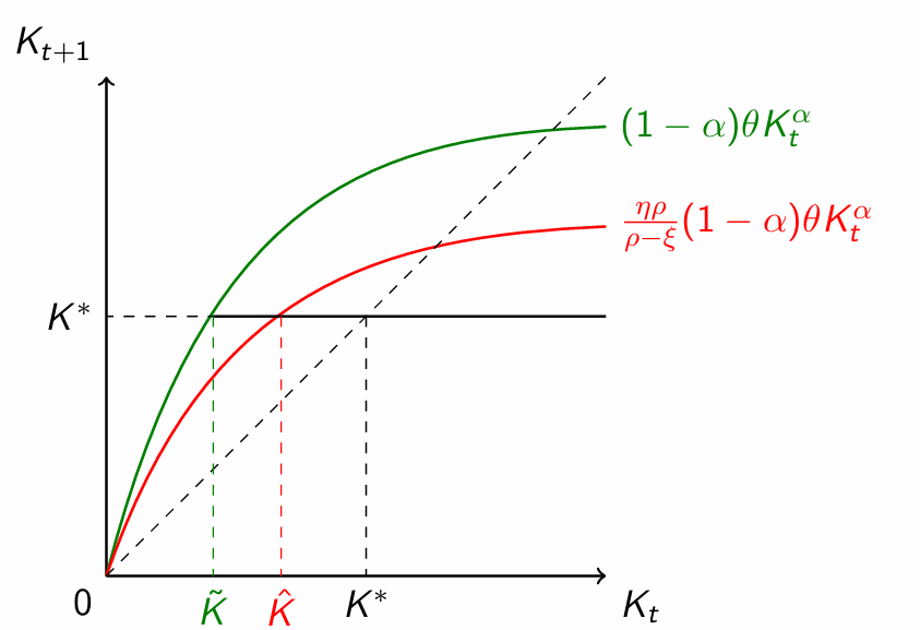
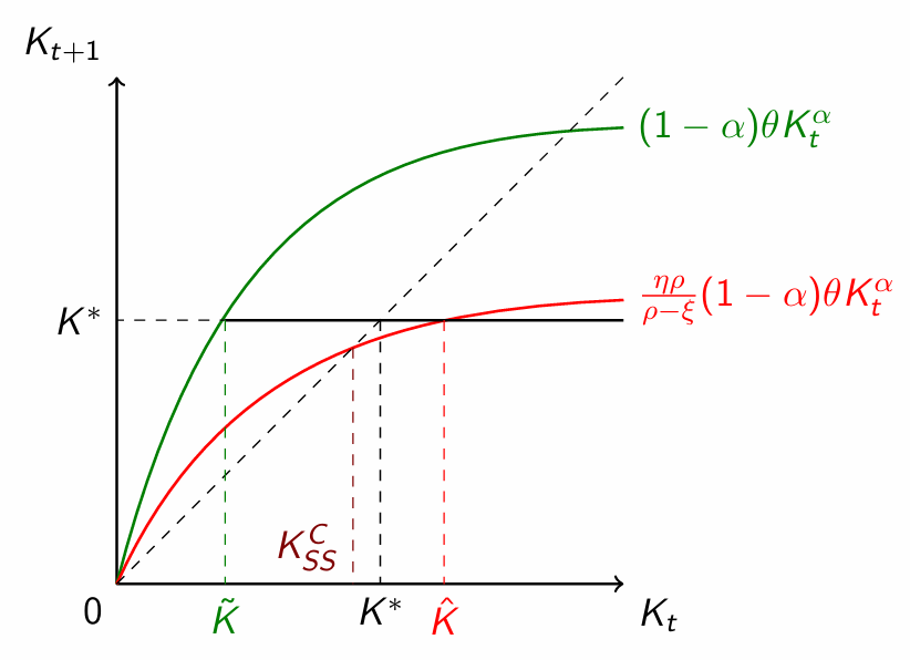
Summing up, financial frictions constrain the ability of the aggregate economy to direct resources into productive capital investments. Starting at a low $K$, an economy subject to frictions grows slower. Moreover, financial frictions can also affect outcomes in the long run, with the economy converging to a steady state with lower economic activity.

Financial Accelerator (Bernanke and Gertler, 1989)

This chapter links business cycle fluctuations to microfounded financial frictions. In fact, the starting point is the idea that financial conditions of banks can have effects on macroeconomic fluctuations, especially booms and crises.

Modigliani-Miller

In the absence of:

• distortionary taxes
• bankruptcy costs
• agency costs and asymmetric information
• inefficient markets⁴

then, the value of a firm or an investment project is unaffecred by how its financed.

This “corporate finance” formulation of the Modigliani-Miller theorem is also known as capital structure irrelevance theorem.

The theorem (whose proof relies on arbitrage opportunities) provides a clear benchmark upon which to build a model, by choosing which specific assumption may not hold in a setting of interest. In modeling, the consequences of the theorem will mainly apply on the choices and behavior of the firms.

Bernanke and Gertler (1989) is the first paper to formally show how financial market conditions can matter for business cycles. Bernanke developed the model motivated by the Great Depression and the disruptions in the (credit) markets that it entailed, in contrast with the prevailing “monteray” view of the Great Depression. Bernanke’s idea is based on asymmetric information: at any point in time, the ability of intermediaries may worsen, affecting the quality of borrowing, investment, and those aggregate outcomes. If the net worth of firms worsens, their access to finance is hindered and triggers a depression: financial intermediaries may stop working when they are needed the most. This view is that financial markets are basically an accelerator of macroeconomic outcomes.

Time is discrete and infinite, with Diamond-fashioned OLG of agents of mass one and two-period lifetimes, and savers and lenders in the same way as in the previous model (preferences are also identical). Returns on storage are now denoted by $r>1$, and units of labor sum to (but can be individually different from) 1 at the aggregate level. Entrepreneurs can store too in this model (in the previous model, lenders faced no financial constraints so entrepreneur could “implicitly” store by lending to the lenders in the debt market). Suppose entrepreneurs face heterogeneous investment costs as a type $\omega \sim \text{U}[0,1]$. Investment is such that $x(\omega )$ units of consumption goods invested at $t$ lead to $\kappa$ units of capital at $t+1$, with $x(\omega )$ increasing in $\omega$ (a cost function increasing the type). Projects are nondivisible: the only investment yielding any outcomes is exactly the entrepreneur-specific unitary investment with cost $x(\omega )$. Moreover, $\kappa \in \{{\kappa }_L,{\kappa }_H\}$ regulated by a transition probability matrix $\pi$. Production follows a Cobb-Douglas technology:

$$F_t(k_{it},l_{it},{\tilde{\theta }}_t)={\tilde{\theta }}_t\cdot k_{it}^{\alpha }\cdot l_{it}^{1-\alpha }$$

where (aggregate) productivity can be assumed to be iid with $\theta \equiv \mathbb{E}[{\tilde{\theta }}_t]$.

Markets for capital and labor are perfectly competitive. As for the credit market, young entrepreneurs can borrow from lenders $b_t$ and invest $S_t^E+b_t$ — a mixture of self-finance and borrowing. Of course, they need to compensate the lenders for the opportunity cost $r$ (the interest rate) during the next period, and competitive forces will always push down returns down to equalize $r$. Contracts are state-contingent on the stochastic realization $\kappa$, but there is asymmetric information about $\kappa$ as the main friction in this economy. In particular, entrepreneurs observe $\kappa$, while lenders can only observe it by auditing the project at a cost of $\gamma \ge 0$ units of capital. Suppose an entrepreneur borrowed $b_t$ and promised to repay $\{R_{t+1}(\kappa )\}$, and make the additional assumption that the contract is settled, at $t+1$, before the TFP shock ${\tilde{\theta }}_{t+1}$ is realized (otherwise, borrowers could start making contract on such realization too). The entrepreneur has the opportunity to observe $\kappa$ and yet misreport $\hat{\kappa }$. If not audited, then the entrepreneur repays $R_{t+1}(\hat{\kappa })$. If audited, instead, $\kappa$ becomes public and the entrepreneur repays $R_{t+1}(\kappa )$. Lenders should, of course, pay for the auditing cost: a $\gamma$ loss of capital at $t+1$ is valued ${\hat{q}}_{t+1}\gamma$ in period $t$, where ${\hat{q}}_{t+1}\equiv \mathbb{E}[r_{t+1}^K]=\theta \alpha k_{t+1}^{\alpha -1}$ is the utility value of capital before production and before the TFP realization. An important point to make is that the contracts are getting settled at the beginning of the period, where TFP is not realized nor production has taken place. Therefore, the resources available to the entrepreneur to repay the lender is constrained by $\kappa {\hat{q}}_{t+1}$.

When solving this contract, we may want to apply the ^b91121 and focus on truthtelling contracts. The contracts will not only include two numbers: they are functions of what was the reported $\kappa$, what was the true $\kappa$, and whether the borrower was audited. There are six total combination: the four combinations of $\{{\kappa }_L,{\kappa }_H\}$ in case of auditing, and the two cases where the borrower is not audited⁵.

Benchmark without asymmetric information

Assume $\gamma =0$, meaning that the entreprenur has no incentive to lie as auditing is always carried out. First, suppose that $S_t^E>x(\omega )$ and the entrepreneur can self-finance. Thye compare two possibilities:

• Investing $x(\omega )$ to get $[\underset{{\kappa }^e}{\underbrace{\pi {\kappa }_H+(1-\pi ){\kappa }_L}}]{\hat{q}}_{t+1}$
• Store $x(\omega )$ and get $rx(\omega )$ Therefore, investment is carried out if and only if ${\kappa }^e{\hat{q}}_{t+1}\ge rx(\omega )$, which is equivalent to if and only if $\omega \le \bar{\omega }$ such that ${\kappa }^e{\hat{q}}_{t+1}=rx(\bar{\omega })$.

Second, consider the extreme of an entrepreneur with no net-worth, that is $S_t^E=0$. Then, they must borrow from lenders to fund their investment: they borrow $x(\omega )$ and invest expecting to get ${\kappa }^e{\hat{q}}_{t+1}$. Since lenders always audit (there is no cost in doing so), the entrepreneur cannot misreport and always pays what’s due, so that repayment must satisfy

$$\pi R({\kappa }_H)+(1-\pi )R({\kappa }_L)\ge rx(\omega )$$

where the RHS is the outside option (be it storage or competitive credit market). As a second constraint, it must be that ${\kappa }_j{\hat{q}}_{t+1}\ge R({\kappa }_j)$ of each level $j\in \{L,H\}$. This suggests that there is no benefit in raising funds to store, as the returns for these two activities will be the same. The entrepreneur receives from this kind of contract the expected payoff

$$\pi [{\hat{q}}_{t+1}{\kappa }_H-R({\kappa }_H)]+(1-\pi )[{\hat{q}}_{t+1}{\kappa }_L-R({\kappa }_L)]={\kappa }^e{\hat{q}}_{t-1}-[\pi R({\kappa }_H)+(1-\pi )R({\kappa }_L)]$$

Because of competitive forces, the participation constraint of the lender will always hold with equality, and therefore the expected payoff of the entrepreneur is ultimately equal to ${\kappa }^e{\hat{q}}_{t+1}-rx(\omega )$. Note that:

• If this is negative, the entrepreneur cannot and do not want to invest (the repayment exceeds the returns in expectation).
• If positive, then it is possible to set $R({\kappa }_j)={\kappa }_j{\hat{q}}_{t+1}$ (or even better values, such as $R({\kappa }_j)<{\kappa }_j{\hat{q}}_{t+1}$). Ultimately, the way the entrepreneur is financed is completely irrelevant for their investment decision, which simply complies to:

$${\kappa }^e{\hat{q}}_{t+1}\ge rx(\omega )⟺\omega \le \bar{\omega }$$

that means that net worth does not matter for investing decisions.

The equilibrium in this benchmark version requires to combine capital demand and supply. The (inverse) demand schedule for capital is given by the price of capital before the TFP realization: ${\hat{q}}_{t+1}=\theta \alpha k_{t+1}^{\alpha -1}$. All entrepreneurs $\omega \le \bar{\omega }$ invest, so the number of projects invested is $\eta \bar{\omega }$, leading to the expected capital supply: $k_{t+1}={\kappa }^e\bar{\omega }\eta$. Note that:

$$rx(\bar{\omega })={\kappa }^e{\hat{q}}_{t+1}⟺\bar{\omega }=x^{-1}\left(\frac{{\kappa }^e{\hat{q}}_{t+1}}{r}\right)$$

The equilibrium is given by the intersection of the two schedules:

$$\begin{array}{rlr}{\hat{q}}_{t+1}& =\theta \alpha k_{t+1}^{\alpha -1}& [\text{DD}]\\ k_{t+1}& ={\kappa }^e\bar{\omega }\eta & [\text{SS}]\end{array}$$

in the $(k_{t+1},{\hat{q}}_{t+1})$-space. Productivity shocks ${\tilde{\theta }}_t$ have no effect on investment, but affect young generation’s wages. It is, however, implicitly assume that such wages are still enough to fund investment.

Benchmark with extreme auditing costs

By contrast, suppose now that $\gamma =\infty$, where no auditing ever takes place. Entrepreneurs will always report so as to minimize their payments, so that contracts cannot be contingent on $\kappa$: whatever the borrower reports, the lender cannot verify it, and for any $\kappa$ actually realized the report will always be the lowest possible. Therefore, $R({\kappa }_H)=R({\kappa }_L)\equiv \bar{R}$.

• If $S_t^E\ge x(\omega )$, the entrepreneur invests on her own if and only if $\omega \le \bar{\omega }$.
• If $S_t^E<x(\omega )$, the entrepreneur must borrow $b=x(\omega )-S_t^E$ to invest. For lenders to be willing to lend:

$$\underset{\equiv \bar{R}}{\underbrace{\pi R({\kappa }_H)+(1-\pi )R({\kappa }_L)}}\ge rb=[x(\omega )-S_t^E]$$

Yet, to be able to pay back what is promised, it must be that ${\kappa }_j{\hat{q}}_{t+1}\ge \bar{R}$ for all realizations $j\in \{L,H\}$. Since ${\kappa }_L<{\kappa }_H$, the entrepreneur can only borrow if ${\kappa }_L^e{\hat{q}}_{t+1}\ge r[x(\omega )-S_t^E]$. However, it is still the case that the entrepreneur is willing to invest. The expected utility from investing is equal to ${\kappa }^e{\hat{q}}_{t+1}-\bar{R}={\kappa }^e{\hat{q}}_{t+1}-r[x(\omega )-S_t^E]$ for any entrepreneur with net worth $S_t^E$, which exceeds the utility from storage (the outside option for lenders, $r{S}_t^E$) if and only if ${\kappa }^e{\hat{q}}_{t+1}\ge rx(\omega )⟺\omega \le \bar{\omega }$. That is, the inability to monitor raises constraints on which entrepreneurs can potentially borrow; however, once the project has been initialized, the repayment is still equal to the original outside option. Put simply, the entrepreneur is able and willing to invest if and only if $\omega \le {\omega }^{\ast }$ where $rx({\omega }^{\ast })=\min \{{\kappa }^e{\hat{q}}_{t+1},{\kappa }_L{\hat{q}}_{t+1}+r{S}_t^E\}$. If the RHS is the minimum of the set, then higher net worth entrepreneurs invest (up to a point), and net worth matters for investment. In fact, the maximum amount that can be promised to any lender is pinned down by the lowest type. Thus, if the levels are very far apart, with financial frictions investment is limited by ${\kappa }_L$. To determine the capital stock, use the same method as before, drawing demand and supply for capital.

Finally, consider the intermediate case where $\gamma \in (0,\infty )$. For reasonable values of $\gamma$, lenders may want to audit when entreprenurs report failure. Just as before, types $\omega \le {\omega }^{\ast }$ borrow non-contingent contracts that do not involve auditing, to avoid auditing costs. Consider type $\omega >{\omega }^{\ast }$ and suppose that lenders extend credit and audit entrepreneurs when they report ${\kappa }_L$. When lenders audit, entrepreneurs have no incentive to misreport. Since monitoring is taken place, lenders incur the monitoring cost:

$$\pi R({\kappa }_H)+(1-\pi )[R({\kappa }_L)-\gamma {\hat{q}}_{t+1}]\ge r(x(\omega )-S_t^E)$$

At equality, thanks to competition in the lending market, the previous condition implies that the expected returns to the entrepreneurs are equal to

$${\kappa }^e{\hat{q}}_{t+1}-r(x(\omega )-S_t^E)-(1-\pi )\gamma {\hat{q}}_{t+1}$$

where the last element on the RHS is the expected monitoring cost. This is preferred to storage, with return $r{S}_t^E$, if and only if:

$${\kappa }^e{\hat{q}}_{t+1}-(1-\pi )\gamma {\hat{q}}_{t+1}\ge rx(\omega )$$

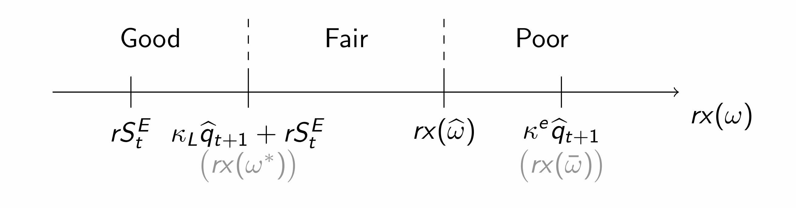
Everything boils down to comparing the entire size of the pie compared to the total opportunity cost of the project. In fact, the lending is happening at the risk free rate, so the effective opportunity cost of running a project is the same for all entrepreneurs. This allows to define a type $\hat{\omega }$ who is indifferent between running a project and storing; note that $\hat{\omega }<\bar{\omega }$ (i.e., the indifferent type is lower when monitoring costs need not be covered). Entrepreneurs can be grouped in three types:

• Good: types $\omega \le {\omega }^{\ast }$ borrow at the riskless interest rate or self-finance if $x(\omega )\le S_t^E$
• Fair: types $\omega \in ({\omega }^{\ast },\hat{\omega }]$ must compensate lenders also for the auditing cost.
• Poor: types $\omega >\hat{\omega }$ are excluded from the market and do not invest (in principle, they could write contract, but with payoff inferior to the sheer storage) The composition of entrepreneurs between the three types depends on $S_t^E$.

For greater $S_t^E$, more entrepreneur switch from suffering from monitoring cost to contracts without monitoring, saving up capital and leading to an increase in the supply of capital.

Collateral Amplification Mechanism (Kiyotaki and Moore, 1997)

Asset prices comove significantly with the business cycle. Are these fluctuations a byproduct of the business cycle, or is it the case that the fall in asset prices in bad times actually deepens recessions? This may happen by inducing a decrease in the net worth of agents holding these assets. Assets act as collateral supporting repayment, but are also inputs of production. These amplification narratives may also contribute evidence to the idea why small shocks can induce large effects, and is key in the literature on macroprudential regulation (Lorenzoni, 2008).

Assume one group of agents cannot borrow as much as it likes, because it would otherwise exhibit opportunistic behavior. The borrower faces a collateral/credit constraint: $R_{t+1}{b}_t\le q_{t+1}{k}_t$, where $q_{t+1}$ is the price of the asset (land? capital? opt for land to neglect depreciation) at $t+1$, whereas the stock used as collateral is $k_t$. Note that:

• In the previous specification, borrowing is against the entire capital stock. A fraction could be specified by including $\xi \in (0,1]$.
• Nevertheless, borrowing is already constrained: despite borrowing against the entire capital stock, it is not possible to borrow against the attending (expected) returns from capital. The interdependence of the prices of collateralized assets and credit limits is such that $k_t$ is both used to ensure repayment and to produce output at $t+1$! This powerful mechanism causes the effects of shocks to persist and amplify.

Warning

Note we can no longer use 2OLG models. In fact, for their net worth to be a function of the asset, they need to be holder of that asset in the upcoming period. However, with 2-period agents, their initial net worth includes wages and thus their entire net worth is independent of assets, unless a third period is introduced. Focus on 3+OLG models, or assume that individuals inherit some assets at time 1.

Consider the simplified Krishnamurthy (2003) version of the KM model. Consider three periods $t=0,1,2$ with two goods: perishable corn and durable land. Agents may be farmers or bankers with unit mass and preferences:

$$U^j=\mathbb{E}[c_0^j+c_0^j+c_2^j]$$

where consumption is in terms of corn. Also assume that farmers are poor with endowment ${\omega }_0^F>0$ at $t=0$ while bankers are rich and have large endouwments of corn ${\omega }_t^B\gg 0$ in every period. Bankers are the only capital owners for $\bar{K}>0$.

Both type of agents have access to a production technology producing corn across periods. There is a type-specific productivity term $z_{t+1}^j$, and the production function is increasing over the minimum of the amount of land put into place and corn divided by $\alpha$: put simply, in order to make use of one unit of land, it is necessary to put into place also $\alpha C_t^j$.

$$Y_{t+1}^j=z_{t+1}^j\cdot f^j\left(\min \left\{k_t^j,\frac{C_t^j}{\alpha }\right\}\right)$$

In what follows, assume that the quantity of corn is chosen optimally for any level of invested $k$. Other assumption include:

• $f^j(x)=f(x)=x(A-x)$ for all types with $\bar{K}<A+\alpha <2\bar{K}$. That is, production is a quadratic function, and we work only with its increasing portion.
• $z_1^B=z_2^B=z_2^F=\mathbb{E}[z_1^F]=1$. This implies that farmers’ productivity at time 1 is subject to stochastic shocks, that we consider only in the aggregate. The only source of uncertainty lies in farmer’s productivity at $t=1$.

The market for land is perfectly competitive, with prize $q_0$ at $t=0$, $q_1(z)$ at state $z$ period $t=1$, and finally $q_2(z)=0$ since land cannot be used in the next period and becomes worthless. Farmers can borrow from bankers in the credit market: the key assumption is that they borrow through fully collateralized non-contingent debt contracts. Put simply, if $D_1(z)$ is the amount that farmers promise to repay in period $t=1$ and state $z$, then for all $z$ it holds that $D_1(z)=D\le q_1(z_L)k_0^F$. Since $q_2(z)=0$, it also follows that $D_2(z)=0$. Shutting up credit markets from period 1 to 2 can thus occur without loss of generality, as the only supply of credit would be 0. In what follows, we will guess and verify that the equilibrium gross interest rate is equal to 1. This is due to the preferences of agents, and mostly because bankers are extremely wealthy and exhibit no discounting. For any value different than 1, agents would consume everything at $t=0$ if $R<1$, or at $t=2$ if $R>1$.

Solve the farmer’s problem backwards. At $t=2$, a farmer consumes $c_2^F(z)=f(k_1^F(z))$. At $t=1$ and state $z$, a farmers chooses $k_1^F(z)$ to solve the maximization problem:

$$J^z(w_1(z))\equiv \underset{k_1^F(z)}{\max }{w}_1(z)-(\alpha +q_1(z))k_1^F(z)+f(k_1^F(z))\text{ subject to }\{\begin{array}{l}(\alpha +q_1(z))k_1^F(z)\le w_1(z)\end{array}$$

with $w_1(z)=zf(k_0^F)+q_1(z)k_0^F-D$ denoting the farmer’s net worth (and putting a non-negative constraint on consumption), and plugging in the farmer’s budget at $t=1$. The funds come from the production of corn at time 0 with productivity $z$ plus the land acquired in the previous period, minus the debt obligations. The solution is given by:

$$k_1^F(z)=\{\begin{array}{ll}(f^{\prime }{)}^{-1}(\alpha +q_1(z))\equiv k^{\ast }(z)& \text{ if }{w}_1(z)\ge w_1^{\ast }(z)\\ \frac{w_1(z)}{\alpha +q_1(z)}& \text{ otherwise}\end{array}$$

where $w_1^{\ast }(z)\equiv (\alpha +q_1(z))k_1^{\ast }(z)\equiv (\alpha +q_1(z))(f^{\prime }{)}^{-1}(\alpha +q_1(z))$ — note that $f^{\prime }$ decreases in $k$ by concavity of $f$. Thus, the farmer’s period $t=1$ value over $w_1(z)$ is:

$$J^z(w_1(z))=\{\begin{array}{ll}{w}_1(z)-w_1^{\ast }(z)+f\left(\frac{w_1^{\ast }(z)}{\alpha +q_1(z)}\right)& \text{ if }{w}_1(z)\ge w_1^{\ast }(z)\\ f\left(\frac{w_1(z)}{\alpha +q_1(z)}\right)& \text{ otherwise}\end{array}$$

The shape depends on whether the farmer is constrained at $t=1$ or not. Put simply, coming to the period with high net worth implies a value function linear in the income value: an extra unit of net worth is simply consumed, any leftover from $w_1^{\ast }$ is consumed. Instead, if the agent is poor, every additional unit is put into production, and no consumption is carried out in that period. Moreover:

$$(J^z{)}^{\prime }(w_1(z))=\{\begin{array}{ll}1& \text{ if }{w}_1(z)\ge w_1^{\ast }(z)\\ f^{\prime }\left(\frac{w_1(z)}{\alpha +q_1(z)}\right)\frac{1}{\alpha +q_1(z)}>1& \text{ otherwise}\end{array}$$

that is, the derivative of the value functions suggests that above the cutoff level the value function is linear, based on the preferences, while the value function below the cutoff level is strictly greater than 1. Why so if the marginal utility of consumption is always 1? Simply because the marginal productivity of investment is higher than 1 unit: the value function inherits the shape of the production function. Finally, at $t=0$, a farmer $k_0^F$ and $D$ to solve:

$$\underset{k_0^F,D}{\max }\mathbb{E}[J^z(w_1(z))]\text{ subject to }\{\begin{array}{l}(\alpha +q_0)k_0^F\le D+w_0^F\\ D\le q_1(z_L)k_0^F\end{array}$$

although we will mainly focus on values from time 1 onwards. This equation implicitly assumes that $c_0^F=0$: potentially, the farmer might be financially constrained at $t=1$ with positive probability, and since the interest rate is equal to 1 in equilibrium, consuming in time 0 is never wanted, as avoiding consumption saves as much as possible for the upcoming constraint (and there is no discounting).

To continue, solve the bankers’ problem, which is much simple due to richness and unconstrainedness. At time $t=2$ a banker simply consumes $c_2^B(z)=f(k_1^B(z))+{\omega }_2^B$. At time $t=1$, instead, the bankers solves:

$$\underset{k_1^B(z)}{\max }{w}_1^B(z)-(\alpha -q_1(z))k_1^B(z)+f(k_1^B(z))+{\omega }_2^B\text{ subject to}\{\begin{array}{l}(\alpha +q_1(z))k_1^B(z)\le w_1^B(z)\end{array}$$

Assuming that $w_1^B(z)$ is so large that the constraint never binds:

$$\underset{k_1^B(z)}{\max }-(\alpha +q_1(z))k_1^B(z)+f(k_1^B(z))$$

which is solved for $k_1^B(z)=(f^{\prime }{)}^{-1}(\alpha +q_1(z))\equiv k_1^{\ast }(z)$. Last, at $t=0$ a banker chooses $k_0^B$ to solve:

$$\underset{k_0^B}{\max }-(\alpha +q_0)k_0^B+f(k_0^B)+\mathbb{E}[q_1(z)]k_0^B$$

which is solved for $k_0^B=(f^{\prime }{)}^{-1}(\alpha +q_0-\mathbb{E}[q_1(z)]$, once again assuming that the constraint $c_0^B\ge 0$ is irrelevant and the banker does not want to borrow in the credit market (they are indifferent between $c_0^B$ and $D^B$ at the margin so that $D^B\le q_1(z_L)k_0^B$ is irrelevant).

Equilibrium

All markets must clear; while good market clears by Walras’ law, for the land market and the credit market the following must hold respectively:

$$\{\begin{array}{l}{k}_0^F+k_0^B=\bar{K}\\ k_1^F(z)+k_1^B(z)=\bar{K}\\ {\omega }_0^F+{\omega }_0^B>\alpha \bar{K}\\ {\omega }_1^B+zf(k_0^F)+f(k_0^B)>\alpha \bar{K}\end{array}$$

where credit market clearance is defined as $D_t(z)+D_t^B(z)=0$ at the guessed interest rate 1.

Without frictions, by ^fa03a6, the agents’ net worth is irrelevant for their investment. Thus:

$$\begin{array}{rlr}\alpha +q_1(z)=f^{\prime }(k_1^j(z))& ⟹k_1^j=\frac{\bar{K}}{2}& [t_0]\\ \alpha +q_0=f^{\prime }(k_0^j)+\mathbb{E}[q_1(z)]& ⟹k_0^j=\frac{\bar{K}}{2}& [t_1]\end{array}$$

Thus, in the frictionless economy, land is distributed equally maximizing expected output. Shocks to $z$ only affect consumption at $t=1$. The amount invested by bankers and farmers is identical due to strictly decreasing returns. (Note that the function should be $\mathbb{E}[z_1]f^{\prime }(k_0^j)$, but we assumed such expectation to be 1).

Take $k_0^F$ and $D$ as given, and note that the farmers’ net worth at time 1 is increasing in $q_1(z)$, since $w_1(z)=zf(k_0^F)+q_1(z)k_0^F-D$. This is at the core of the amplification mechanism. At the same time, if farmers happent o be constrained, theire demand for $k$ is increasing in income:

$$k_1^F(z)=\frac{w_1(z)}{\alpha -q_1(z)}$$

increasing in $w_1(z)$. However, the $q_1(z)$ implied by the “supply curve” they face, that is, $\bar{K}-k_1^F(z)$, is also increasing in $k_1^F(z)$. By the bankers’ demand and market clearing;

$$\begin{array}{rl}{q}_1(z)& =f^{\prime }(k_1^B(z))-\alpha \\ & =f^{\prime }(\bar{K}-k_1^F(z))-\alpha \\ & =A-\alpha -2(\bar{K}-k_1^F(z))\end{array}$$

The relationship imposing bankers’ optimality and land market clearing is an upward sloping line in the amount of land held by the farmers. In fact, $k_1^F(z)=\bar{K}-k_1^B(z)$ — the land not hold by bankers must be hold by farmers. If bankers have excess land, their value is reduced and thus they supply more to offset the decrease in its marginal return. Eventually, ^5d3cb9 and ^c89b3d suffice in pinpointing the equilibrium in the land market. When the $L$ state hits and $z=0$, there are two effects:

1. Farmers’ net worth declines as output is lower (technological effect)
2. The price of land declines (amplification effect) In fact, market clearing for $w_1(z)<w_1^{\ast }$ implies:

$$q_1(z)=A-\alpha -2\bar{K}+2\underset{=k_1^F(z)}{\underbrace{\frac{w_1(z)}{\alpha +q_1(z)}}}$$

This general equilibrium amplification is at the hard of the model. The RHS is decreasing in $q_1(z)$, so: if the ability to afford land by the farmers decreases, bankers must buy more, pushing down $q_1$, which in turn also pushes down the net worth of the farmer. This extra hit is the channel of amplification. Bankers’ are “princing the land”: being financially unconstrained, whenever land prices need to adjust, this is done to lead the bankers to buy such land. This mechanism kicks in only when farmers are constrained (if they are unconstrained, the frictionless solution holds, which is also the most efficient production frontier given the strict concavity of technology).

Kiyotaki and Moore argue that this amplification effect can be quite large: in the dynamic extension of this model, the effect will be even stronger, since in the KM world the present price of land corresponds to the infinite discounted future stream of prices: $q_t={\sum }_{j=0}^{\infty }\frac{1}{R^j}{u}_{t+j}$. Moreover, the price shows up in the borrowing constraint, also reducing investment and providing an additional source of amplification.

Footnotes

1. The goods market clear by Walras’ Law. ↩ ↩²

2. The slides (slide 27 from Lecture 2 on Incomplete Markets) erroneusly reported $w(r)=(1-\alpha ){\theta }^{\frac{1}{1-\alpha }}{\left(\frac{\alpha }{r+\delta }\right)}^{\frac{\alpha }{1-\alpha }}$. ↩

3. Recall that, by assumption, $\eta \xi <\xi <(1-\eta )\rho$. ↩

4. The theorem holds with incomplete markets, so far as these are frictionless. ↩

5. The generalization for $n$ levels of $\kappa$ is a set of contracts of size $n^2+n$. An alternative factorial generalization can be thought as based on the permutation $n^2+n=P(n+1,2)=\frac{(n+1)!}{(n-1)!}$. ↩